Recommendation Systems (7): Graph Neural Networks and Social Recommendation

permalink: "en/recommendation-systems-7-graph-neural-networks/" date: 2024-06-01 10:30:00 tags: - Recommendation Systems - GNN - Social Recommendation categories: Recommendation Systems mathjax: true --- When Netflix recommends a movie, it's not just looking at what you've watched — it's analyzing a complex web of relationships: which movies are similar to each other, which users share your taste, and how these connections form patterns across millions of interactions. This intricate network of relationships is exactly what graph neural networks (GNNs) excel at modeling. Unlike traditional recommendation approaches that treat users and items as isolated entities, GNNs capture the rich structural information encoded in user-item interaction graphs, social networks, and knowledge graphs.

Graph neural networks have revolutionized recommendation systems by explicitly modeling the graph structure underlying collaborative filtering. From the foundational Graph Convolutional Networks (GCN) that aggregate neighbor information, to Graph Attention Networks (GAT) that learn adaptive importance weights, to GraphSAGE that enables inductive learning on large-scale graphs, GNNs provide a principled framework for leveraging relational data in recommendations. In recommendation systems, these techniques have given rise to models like PinSage (Pinterest's billion-scale recommender), LightGCN (a simplified yet powerful approach), and NGCF (Neural Graph Collaborative Filtering) that achieve state-of-the-art performance by learning high-quality embeddings through graph convolution operations.

This article provides a comprehensive exploration of graph neural networks for recommendation, covering foundational GNN architectures (GCN, GAT, GraphSAGE), graph modeling strategies for recommendation scenarios, key models (PinSage, LightGCN, NGCF), social recommendation techniques, graph sampling methods for scalability, training strategies, implementation details with 10+ code examples, and detailed Q&A sections addressing common questions and practical challenges.

Why Graph Neural Networks for Recommendation?

The Graph Structure of Recommendation Data

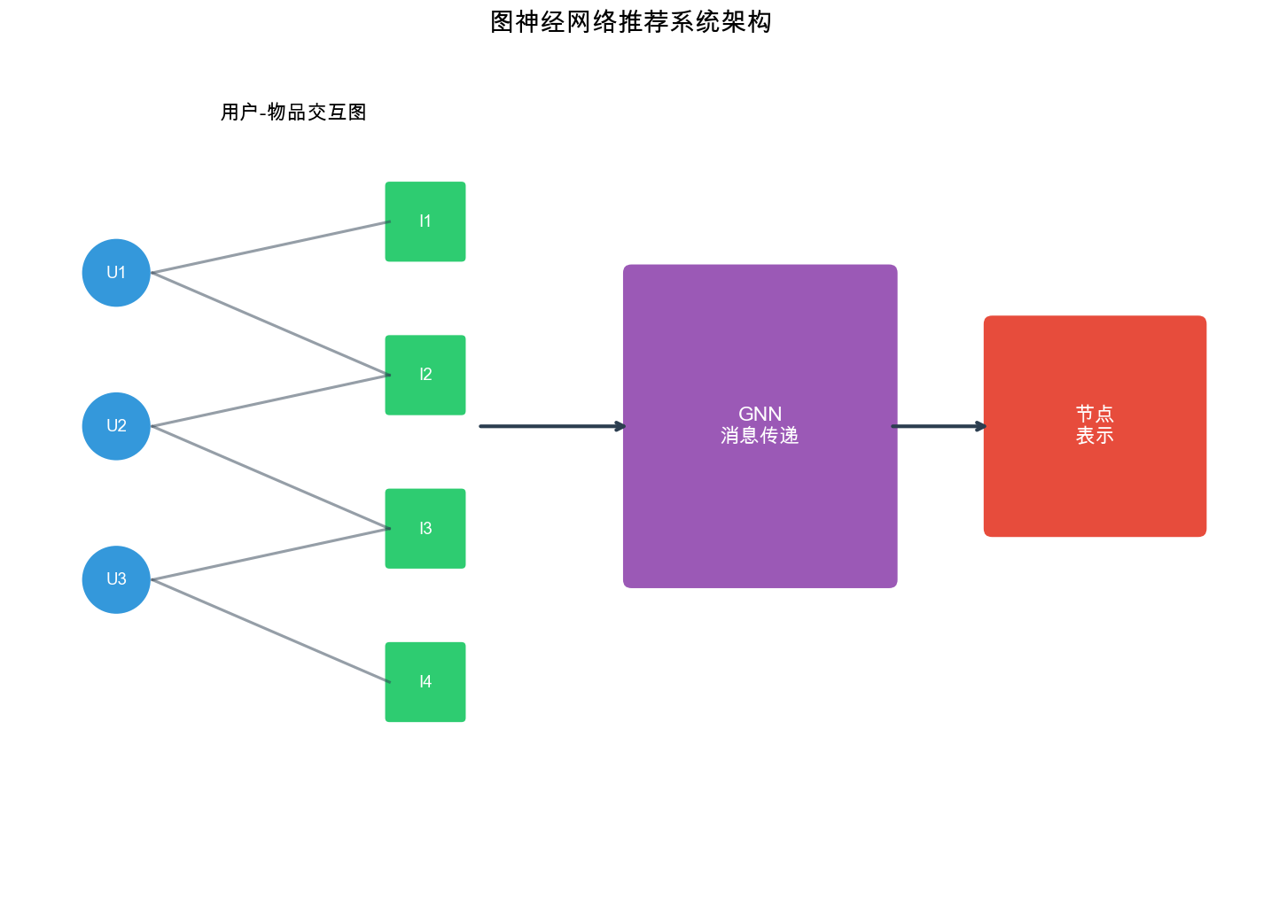
Recommendation systems naturally operate on graph-structured data. Consider a user-item interaction matrix: each row represents a user, each column represents an item, and each entry indicates an interaction (click, purchase, rating). This matrix can be viewed as a bipartite graph where: - Nodes are users and items - Edges represent interactions (with optional weights/features) - The graph structure encodes collaborative signals: users with similar interaction patterns are implicitly connected through shared items

Example: In a movie recommendation scenario: - User \(u_1\)watched movies\(m_1\),\(m_2\),\(m_3\) - User\(u_2\)watched movies\(m_2\),\(m_3\),\(m_4\) - The graph structure reveals that\(u_1\)and\(u_2\)share preferences (through\(m_2\)and\(m_3\)), even if they never directly interacted

Limitations of Traditional Approaches

Traditional collaborative filtering methods have limitations when dealing with graph-structured data:

Matrix Factorization: Learns low-dimensional embeddings but doesn't explicitly model the graph structure. The collaborative signal is implicit in the dot product\(u_i^T v_j\), but there's no mechanism to aggregate information from neighboring nodes.

Deep Learning Approaches: Neural collaborative filtering and autoencoders can capture non-linear patterns but still treat interactions as independent, missing the structural relationships encoded in the graph.

Graph-Agnostic Embeddings: Traditional methods learn embeddings independently for each user/item, ignoring that similar users/items should have similar embeddings based on their graph neighborhoods.

Advantages of Graph Neural Networks

GNNs address these limitations by:

1. Explicit Graph Modeling: Directly operate on the graph structure, allowing models to leverage topological information
2. Neighborhood Aggregation: Aggregate information from neighboring nodes, enabling collaborative signal propagation
3. Multi-Hop Reasoning: Through multiple layers, GNNs can capture multi-hop relationships (e.g., "users who liked items similar to items you liked")
4. Inductive Learning: Some GNN variants (like GraphSAGE) can generalize to unseen nodes, crucial for handling new users/items
5. Heterogeneous Graphs: Can model complex relationships including social networks, knowledge graphs, and item attributes

Graph Neural Network Fundamentals

Graph Basics

A graph\(G = (V, E)\)consists of: - Vertices (Nodes):\(V = \{v_1, v_2, \dots, v_n\}\)representing entities (users, items) - Edges:\(E \subseteq V \times V\)representing relationships (interactions, similarities) - Adjacency Matrix:\(A \in \{0,1\}^{n \times n}\)where\(A_{ij} = 1\)if edge\((v_i, v_j)\)exists

For recommendation, we typically work with: - Bipartite Graphs:\(G = (U \cup I, E)\)where\(U\)are users,\(I\)are items, and edges only connect users to items - Weighted Graphs: Edges have weights (e.g., rating scores, interaction frequencies) - Attributed Graphs: Nodes/edges have feature vectors

Message Passing Framework

GNNs operate through message passing: nodes aggregate information from their neighbors to update their representations. The general framework:

1. Message Computation: Each node computes messages to send to neighbors
2. Message Aggregation: Each node aggregates messages received from neighbors
3. Node Update: Each node updates its representation based on aggregated messages

Formally, for node\(v\)at layer\(l\):\[\mathbf{m}_v^{(l)} = \text{AGGREGATE}^{(l)}(\{\mathbf{h}_u^{(l-1)} : u \in \mathcal{N}(v)\})\] \[\mathbf{h}_v^{(l)} = \text{UPDATE}^{(l)}(\mathbf{h}_v^{(l-1)}, \mathbf{m}_v^{(l)})\]where\(\mathcal{N}(v)\)is the neighborhood of\(v\),\(\mathbf{h}_v^{(l)}\)is the representation of\(v\)at layer\(l\), and\(\text{AGGREGATE}\)and\(\text{UPDATE}\)are learnable functions.

Graph Convolutional Networks (GCN)

Spectral Convolution

GCN was introduced by Kipf & Welling (2017) as a spectral approach to graph convolution. The key idea is to define convolution in the spectral domain (eigenvalue decomposition of the graph Laplacian) and then approximate it efficiently.

The graph Laplacian is defined as:\[L = D - A\]where\(D\)is the degree matrix (\(D_{ii} = \sum_j A_{ij}\)). The normalized Laplacian is:\[L_{\text{norm}} = D^{-\frac{1}{2}} (D - A) D^{-\frac{1}{2}} = I - D^{-\frac{1}{2}} A D^{-\frac{1}{2}}\]

GCN Layer

A GCN layer performs the following operation:\[\mathbf{H}^{(l+1)} = \sigma(\tilde{D}^{-\frac{1}{2}} \tilde{A} \tilde{D}^{-\frac{1}{2}} \mathbf{H}^{(l)} \mathbf{W}^{(l)})\]where: -\(\tilde{A} = A + I\) (add self-loops) -\(\tilde{D}_{ii} = \sum_j \tilde{A}_{ij}\) (degree matrix with self-loops) -\(\mathbf{H}^{(l)} \in \mathbb{R}^{n \times d_l}\)is the node feature matrix at layer\(l\) -\(\mathbf{W}^{(l)} \in \mathbb{R}^{d_l \times d_{l+1}}\)is a learnable weight matrix -\(\sigma\)is an activation function (e.g., ReLU)

The normalization\(\tilde{D}^{-\frac{1}{2 }} \tilde{A} \tilde{D}^{-\frac{1}{2 }}\)ensures that the aggregation is normalized by node degrees, preventing the exploding gradient problem.

Intuition

The GCN operation can be understood as: 1. Linear Transformation:\(\mathbf{H}^{(l)} \mathbf{W}^{(l)}\)transforms node features 2. Neighborhood Aggregation:\(\tilde{A} \mathbf{H}^{(l)} \mathbf{W}^{(l)}\)aggregates features from neighbors (and self) 3. Normalization:\(\tilde{D}^{-\frac{1}{2 }} \tilde{A} \tilde{D}^{-\frac{1}{2 }}\)normalizes by degrees 4. Non-linearity:\(\sigma\)applies activation

For a single node\(v\), the update is:\[\mathbf{h}_v^{(l+1)} = \sigma\left(\sum_{u \in \mathcal{N}(v) \cup \{v} } \frac{1}{\sqrt{d_v d_u }} \mathbf{h}_u^{(l)} \mathbf{W}^{(l)}\right)\]where\(d_v\)is the degree of node\(v\).

Implementation: Basic GCN Layer

import torch
import torch.nn as nn
import torch.nn.functional as F
from torch_geometric.nn import MessagePassing
from torch_geometric.utils import add_self_loops, degree

class GCNLayer(nn.Module):
    """
    Graph Convolutional Network layer.
    """
    def __init__(self, in_channels, out_channels):
        super(GCNLayer, self).__init__()
        self.linear = nn.Linear(in_channels, out_channels)
        
    def forward(self, x, edge_index):
        """
        Args:
            x: Node feature matrix [num_nodes, in_channels]
            edge_index: Graph connectivity [2, num_edges]
        Returns:
            Updated node features [num_nodes, out_channels]
        """
        # Add self-loops
        edge_index, _ = add_self_loops(edge_index, num_nodes=x.size(0))
        
        # Compute normalization coefficients
        row, col = edge_index
        deg = degree(col, x.size(0), dtype=x.dtype)
        deg_inv_sqrt = deg.pow(-0.5)
        deg_inv_sqrt[deg_inv_sqrt == float('inf')] = 0
        norm = deg_inv_sqrt[row] * deg_inv_sqrt[col]
        
        # Linear transformation
        x = self.linear(x)
        
        # Message passing: aggregate neighbor features
        out = self.propagate(edge_index, x=x, norm=norm)
        
        return out
    
    def message(self, x_j, norm):
        """
        Compute messages: normalized neighbor features
        """
        return norm.view(-1, 1) * x_j

Multi-Layer GCN

Stacking multiple GCN layers enables the model to capture multi-hop dependencies:

class GCN(nn.Module):
    """
    Multi-layer Graph Convolutional Network.
    """
    def __init__(self, num_nodes, in_channels, hidden_channels, out_channels, num_layers=2, dropout=0.5):
        super(GCN, self).__init__()
        self.num_layers = num_layers
        self.dropout = dropout
        
        # Initialize node embeddings if no input features
        if in_channels == 0:
            self.embedding = nn.Embedding(num_nodes, hidden_channels)
            in_channels = hidden_channels
        else:
            self.embedding = None
        
        # GCN layers
        self.convs = nn.ModuleList()
        if num_layers == 1:
            self.convs.append(GCNLayer(in_channels, out_channels))
        else:
            self.convs.append(GCNLayer(in_channels, hidden_channels))
            for _ in range(num_layers - 2):
                self.convs.append(GCNLayer(hidden_channels, hidden_channels))
            self.convs.append(GCNLayer(hidden_channels, out_channels))
    
    def forward(self, x, edge_index):
        if self.embedding is not None:
            x = self.embedding.weight
        
        # Apply GCN layers
        for i, conv in enumerate(self.convs):
            x = conv(x, edge_index)
            if i < self.num_layers - 1:
                x = F.relu(x)
                x = F.dropout(x, p=self.dropout, training=self.training)
        
        return x

Graph Attention Networks (GAT)

Attention Mechanism

While GCN uses fixed weights based on node degrees, GAT (Veli č kovi ć et al., 2018) learns adaptive attention weights that determine how much importance to assign to each neighbor. This allows the model to focus on more relevant neighbors.

GAT Layer

A GAT layer computes attention coefficients for each edge:\[e_{ij} = \text{LeakyReLU}(\mathbf{a}^T [\mathbf{W}\mathbf{h}_i \| \mathbf{W}\mathbf{h}_j])\]where\(\mathbf{a}\)is a learnable attention vector,\(\mathbf{W}\)is a weight matrix, and\(\|\)denotes concatenation.

The attention coefficients are normalized using softmax:\[\alpha_{ij} = \frac{\exp(e_{ij})}{\sum_{k \in \mathcal{N}(i)} \exp(e_{ik})}\]The node update is then:\[\mathbf{h}_i^{(l+1)} = \sigma\left(\sum_{j \in \mathcal{N}(i) \cup \{i} } \alpha_{ij} \mathbf{W}^{(l)} \mathbf{h}_j^{(l)}\right)\]

Multi-Head Attention

GAT typically uses multi-head attention to stabilize learning:\[\mathbf{h}_i^{(l+1)} = \|{}_{k=1}^{K} \sigma\left(\sum_{j \in \mathcal{N}(i) \cup \{i} } \alpha_{ij}^{(k)} \mathbf{W}^{(k)} \mathbf{h}_j^{(l)}\right)\]where\(K\)is the number of attention heads and\(\|\)denotes concatenation. For the final layer, averaging is often used instead of concatenation.

Implementation: GAT Layer

import torch
import torch.nn as nn
import torch.nn.functional as F
from torch_geometric.nn import MessagePassing
from torch_geometric.utils import add_self_loops

class GATLayer(MessagePassing):
    """
    Graph Attention Network layer.
    """
    def __init__(self, in_channels, out_channels, heads=1, dropout=0.0, concat=True):
        super(GATLayer, self).__init__(aggr='add', node_dim=0)
        self.in_channels = in_channels
        self.out_channels = out_channels
        self.heads = heads
        self.concat = concat
        self.dropout = dropout
        
        # Linear transformation for each head
        self.lin = nn.Linear(in_channels, heads * out_channels, bias=False)
        
        # Attention mechanism: learnable parameters
        self.att = nn.Parameter(torch.empty(1, heads, 2 * out_channels))
        
        self.reset_parameters()
    
    def reset_parameters(self):
        nn.init.xavier_uniform_(self.lin.weight)
        nn.init.xavier_uniform_(self.att)
    
    def forward(self, x, edge_index):
        """
        Args:
            x: Node features [num_nodes, in_channels]
            edge_index: Graph connectivity [2, num_edges]
        """
        # Add self-loops
        edge_index, _ = add_self_loops(edge_index, num_nodes=x.size(0))
        
        # Linear transformation
        x = self.lin(x).view(-1, self.heads, self.out_channels)
        
        # Start message passing
        out = self.propagate(edge_index, x=x)
        
        if self.concat:
            out = out.view(-1, self.heads * self.out_channels)
        else:
            out = out.mean(dim=1)
        
        return out
    
    def message(self, x_i, x_j, edge_index_i):
        """
        Compute messages with attention weights.
        """
        # Compute attention scores
        x_i = x_i.view(-1, self.heads, self.out_channels)
        x_j = x_j.view(-1, self.heads, self.out_channels)
        
        # Concatenate and compute attention
        alpha = (torch.cat([x_i, x_j], dim=-1) * self.att).sum(dim=-1)
        alpha = F.leaky_relu(alpha, negative_slope=0.2)
        alpha = self.edge_updater(alpha, edge_index_i)
        
        # Apply attention weights
        return x_j * alpha.view(-1, self.heads, 1)
    
    def edge_updater(self, alpha, edge_index_i):
        """
        Normalize attention scores using softmax.
        """
        # Softmax over neighbors
        alpha = softmax(alpha, edge_index_i)
        alpha = F.dropout(alpha, p=self.dropout, training=self.training)
        return alpha

def softmax(src, index, num_nodes=None):
    """
    Sparse softmax: normalize attention scores per node.
    """
    num_nodes = index.max().item() + 1 if num_nodes is None else num_nodes
    out = src - scatter_max(src, index, dim=0, dim_size=num_nodes)[0][index]
    out = out.exp()
    out = out / (scatter_add(out, index, dim=0, dim_size=num_nodes)[index] + 1e-16)
    return out

def scatter_max(src, index, dim=0, dim_size=None):
    """Helper function for sparse max."""
    return torch_scatter.scatter_max(src, index, dim=dim, dim_size=dim_size)

def scatter_add(src, index, dim=0, dim_size=None):
    """Helper function for sparse add."""
    return torch_scatter.scatter_add(src, index, dim=dim, dim_size=dim_size)

GraphSAGE

Inductive Learning

GraphSAGE (Hamilton et al., 2017) addresses a key limitation of GCN: transductive learning. GCN requires the entire graph during training and cannot generalize to new nodes. GraphSAGE enables inductive learning by learning aggregation functions rather than fixed node embeddings.

Sampling and Aggregation

GraphSAGE uses two key ideas:

1. Neighbor Sampling: Instead of using all neighbors, sample a fixed-size neighborhood
2. Aggregation Functions: Learn functions to aggregate sampled neighbor features

The algorithm:

1. Sample Neighbors: For each node, sample\(k\)neighbors at each hop
2. Aggregate: Aggregate features from sampled neighbors using a learned function
3. Combine: Combine aggregated neighbor features with node's own features

Formally, for node\(v\):\[\mathbf{h}_{\mathcal{N}(v)}^{(l)} = \text{AGGREGATE}^{(l)}(\{\mathbf{h}_u^{(l-1)} : u \in \mathcal{N}(v)} )\] \[\mathbf{h}_v^{(l)} = \sigma(\mathbf{W}^{(l)} \cdot [\mathbf{h}_v^{(l-1)} \| \mathbf{h}_{\mathcal{N}(v)}^{(l)}])\]where\(\|\)denotes concatenation.

Aggregation Functions

GraphSAGE supports several aggregation functions:

Mean Aggregator:\[\mathbf{h}_{\mathcal{N}(v)} = \frac{1}{|\mathcal{N}(v)|} \sum_{u \in \mathcal{N}(v)} \mathbf{h}_u\]

LSTM Aggregator: Uses an LSTM to process neighbors (requires ordering)

Pooling Aggregator:\[\mathbf{h}_{\mathcal{N}(v)} = \max(\{\sigma(\mathbf{W}_{\text{pool }} \mathbf{h}_u + \mathbf{b}) : u \in \mathcal{N}(v)} )\]

Implementation: GraphSAGE Layer

import torch
import torch.nn as nn
import torch.nn.functional as F
from torch_geometric.nn import MessagePassing
from torch_geometric.utils import add_self_loops

class SAGEConv(MessagePassing):
    """
    GraphSAGE convolution layer.
    """
    def __init__(self, in_channels, out_channels, aggr='mean', normalize=False):
        super(SAGEConv, self).__init__(aggr='mean')
        self.in_channels = in_channels
        self.out_channels = out_channels
        self.aggr = aggr
        self.normalize = normalize
        
        # Linear transformations
        self.lin_l = nn.Linear(in_channels, out_channels)  # Self features
        self.lin_r = nn.Linear(in_channels, out_channels)  # Neighbor features
    
    def forward(self, x, edge_index):
        """
        Args:
            x: Node features [num_nodes, in_channels]
            edge_index: Graph connectivity [2, num_edges]
        """
        # Add self-loops
        edge_index, _ = add_self_loops(edge_index, num_nodes=x.size(0))
        
        # Propagate messages
        out = self.propagate(edge_index, x=x)
        
        # Combine self and neighbor features
        out = self.lin_l(x) + self.lin_r(out)
        
        if self.normalize:
            out = F.normalize(out, p=2, dim=1)
        
        return out
    
    def message(self, x_j):
        """
        Message: neighbor features
        """
        return x_j

Neighbor Sampling

For large graphs, GraphSAGE uses neighbor sampling to control computational cost:

import torch
from torch_geometric.data import NeighborSampler

class GraphSAGEWithSampling(nn.Module):
    """
    GraphSAGE with neighbor sampling for large-scale graphs.
    """
    def __init__(self, num_nodes, in_channels, hidden_channels, out_channels, num_layers=2):
        super(GraphSAGEWithSampling, self).__init__()
        self.num_layers = num_layers
        
        # Initialize embeddings
        self.embedding = nn.Embedding(num_nodes, hidden_channels)
        
        # SAGE layers
        self.convs = nn.ModuleList()
        if num_layers == 1:
            self.convs.append(SAGEConv(hidden_channels, out_channels))
        else:
            self.convs.append(SAGEConv(hidden_channels, hidden_channels))
            for _ in range(num_layers - 2):
                self.convs.append(SAGEConv(hidden_channels, hidden_channels))
            self.convs.append(SAGEConv(hidden_channels, out_channels))
    
    def forward(self, x, adjs):
        """
        Args:
            x: Node features
            adjs: List of (edge_index, e_id, size) tuples from NeighborSampler
        """
        for i, (edge_index, _, size) in enumerate(adjs):
            x_target = x[:size[1]]  # Target nodes
            x = self.convs[i]((x, x_target), edge_index)
            if i < self.num_layers - 1:
                x = F.relu(x)
                x = F.dropout(x, training=self.training)
        
        return x

Graph Modeling for Recommendation

User-Item Bipartite Graph

The most common graph structure in recommendation is the user-item bipartite graph:

• Nodes: Users\(U = \{u_1, u_2, \dots, u_m\}\)and items\(I = \{i_1, i_2, \dots, i_n\}\)
• Edges: Interactions\((u, i)\)with optional weights (ratings, clicks, purchases)
• Adjacency Matrix:\[A = \begin{bmatrix} 0 & R \\ R^T & 0 \end{bmatrix}\]where\(R \in \mathbb{R}^{m \times n}\)is the user-item interaction matrix

Heterogeneous Graphs

Real-world recommendation often involves heterogeneous graphs with multiple node/edge types:

• Node Types: Users, items, attributes (categories, brands), entities (actors, directors)
• Edge Types: Interactions (click, purchase), relationships (friend, follow), attributes (belongs-to, has)

Example: A movie recommendation graph might have: - User nodes - Movie nodes
- Actor nodes - Genre nodes - Edges: (user, watched, movie), (movie, has_actor, actor), (movie, has_genre, genre)

Knowledge Graphs

Knowledge graphs encode structured knowledge about items:

• Entities: Items, attributes, concepts
• Relations: Semantic relationships (directed_by, produced_by, similar_to)
• Triples: (subject, relation, object)

Example: (The Matrix, directed_by, Wachowskis), (The Matrix, similar_to, Inception)

Knowledge graphs enable explainable recommendations by leveraging semantic relationships.

Multi-Relational Graphs

Some recommendation scenarios involve multi-relational graphs where edges have types:

• Social relations: friend, follow, trust
• Interaction types: view, click, purchase, rate
• Item relations: similar, co-purchased, co-viewed

Each relation type can have different semantics and should be modeled separately.

PinSage: Billion-Scale Recommendation

Overview

PinSage (Ying et al., 2018) is Pinterest's graph convolutional network for web-scale recommendation. It handles graphs with billions of nodes and edges, making it one of the largest GNN applications.

Key Innovations

1. Random Walk Sampling Instead of using all neighbors, PinSage samples important neighbors using random walks:

• Start from target node
• Perform random walks to identify important neighbors
• Use top-\(k\)neighbors by visit frequency

2. Importance-Based Aggregation Aggregate neighbor features weighted by importance scores from random walks:\[\mathbf{h}_v^{(l)} = \sigma(\mathbf{W}^{(l)} \cdot \text{CONCAT}[\mathbf{h}_v^{(l-1)}, \text{AGGREGATE}(\{\alpha_{uv} \mathbf{h}_u^{(l-1)} : u \in \mathcal{N}(v)} )])\]where\(\alpha_{uv}\)is the importance score from random walks.

3. Efficient Training - Negative Sampling: Sample negative items for each positive interaction - Hard Negatives: Use difficult negative examples to improve learning - Multi-GPU Training: Distribute computation across GPUs

Implementation: PinSage Convolution

import torch
import torch.nn as nn
import torch.nn.functional as F
import numpy as np
from collections import Counter

class PinSageConv(nn.Module):
    """
    PinSage convolution layer with importance-based aggregation.
    """
    def __init__(self, in_channels, out_channels):
        super(PinSageConv, self).__init__()
        self.in_channels = in_channels
        self.out_channels = out_channels
        
        # Two-layer MLP for aggregation
        self.aggregator = nn.Sequential(
            nn.Linear(in_channels, out_channels),
            nn.ReLU(),
            nn.Linear(out_channels, out_channels)
        )
        
        # Transformation for concatenation
        self.combine = nn.Linear(in_channels + out_channels, out_channels)
    
    def forward(self, x, edge_index, importance_weights=None):
        """
        Args:
            x: Node features [num_nodes, in_channels]
            edge_index: Graph connectivity [2, num_edges]
            importance_weights: Optional importance weights [num_edges]
        """
        row, col = edge_index
        
        # Aggregate neighbor features
        if importance_weights is not None:
            # Weighted aggregation
            neighbor_features = x[col] * importance_weights.view(-1, 1)
            aggregated = scatter_add(neighbor_features, row, dim=0, dim_size=x.size(0))
        else:
            # Mean aggregation
            neighbor_features = x[col]
            aggregated = scatter_mean(neighbor_features, row, dim=0, dim_size=x.size(0))
        
        # Apply aggregator MLP
        aggregated = self.aggregator(aggregated)
        
        # Combine with self features
        combined = torch.cat([x, aggregated], dim=1)
        out = self.combine(combined)
        
        return out

def compute_random_walk_importance(edge_index, num_nodes, num_walks=10, walk_length=5, top_k=10):
    """
    Compute importance scores using random walks.
    
    Args:
        edge_index: Graph connectivity
        num_nodes: Number of nodes
        num_walks: Number of random walks per node
        walk_length: Length of each walk
        top_k: Number of top neighbors to keep
    
    Returns:
        Dictionary mapping (source, target) -> importance score
    """
    importance_scores = Counter()
    
    # Convert to adjacency list
    adj_list = {}
    row, col = edge_index.cpu().numpy()
    for i in range(len(row)):
        if row[i] not in adj_list:
            adj_list[row[i]] = []
        adj_list[row[i]].append(col[i])
    
    # Perform random walks
    for start_node in range(num_nodes):
        if start_node not in adj_list:
            continue
        
        for _ in range(num_walks):
            current = start_node
            for _ in range(walk_length):
                if current not in adj_list or len(adj_list[current]) == 0:
                    break
                # Random neighbor
                current = np.random.choice(adj_list[current])
                importance_scores[(start_node, current)] += 1
    
    # Normalize and keep top-k
    normalized_scores = {}
    for (source, target), count in importance_scores.items():
        if source not in normalized_scores:
            normalized_scores[source] = []
        normalized_scores[source].append((target, count))
    
    # Keep top-k neighbors per source
    final_scores = {}
    for source, neighbors in normalized_scores.items():
        neighbors.sort(key=lambda x: x[1], reverse=True)
        total_count = sum(count for _, count in neighbors[:top_k])
        for target, count in neighbors[:top_k]:
            final_scores[(source, target)] = count / total_count if total_count > 0 else 0
    
    return final_scores

LightGCN: Simplifying GCN for Recommendation

Motivation

LightGCN (He et al., 2020) simplifies GCN by removing unnecessary components: - No feature transformation: Removes the linear transformation matrix - No non-linear activation: Removes ReLU activation - No self-connection: Removes explicit self-loops (handled by layer combination)

The key insight: feature transformation and non-linearity are not necessary for collaborative filtering — the graph structure itself provides sufficient signal.

LightGCN Architecture

LightGCN uses a simple aggregation rule:\[\mathbf{e}_u^{(l+1)} = \sum_{i \in \mathcal{N}(u)} \frac{1}{\sqrt{|\mathcal{N}(u)| |\mathcal{N}(i)| }} \mathbf{e}_i^{(l)}\] \[\mathbf{e}_i^{(l+1)} = \sum_{u \in \mathcal{N}(i)} \frac{1}{\sqrt{|\mathcal{N}(u)| |\mathcal{N}(i)| }} \mathbf{e}_u^{(l)}\]where\(\mathbf{e}_u^{(l)}\)and\(\mathbf{e}_i^{(l)}\)are user and item embeddings at layer\(l\).

The final embeddings are a weighted combination of all layers:\[\mathbf{e}_u = \sum_{l=0}^{L} \alpha_l \mathbf{e}_u^{(l)}, \quad \mathbf{e}_i = \sum_{l=0}^{L} \alpha_l \mathbf{e}_i^{(l)}\]where\(\alpha_l\)are learnable or fixed weights (often\(\alpha_l = \frac{1}{L+1}\)).

Why LightGCN Works

1. Smoothing Effect: Multiple layers smooth embeddings, bringing similar nodes closer
2. Collaborative Signal: Higher layers capture higher-order collaborative signals
3. Simplicity: Fewer parameters reduce overfitting risk

Implementation: LightGCN

import torch
import torch.nn as nn
import torch.nn.functional as F
from torch_geometric.nn import MessagePassing
from torch_geometric.utils import add_self_loops, degree

class LightGCNLayer(MessagePassing):
    """
    LightGCN layer: simplified GCN without transformation and activation.
    """
    def __init__(self):
        super(LightGCNLayer, self).__init__(aggr='add')
    
    def forward(self, x, edge_index):
        """
        Args:
            x: Node embeddings [num_nodes, embedding_dim]
            edge_index: Graph connectivity [2, num_edges]
        """
        # Compute normalization
        row, col = edge_index
        deg = degree(col, x.size(0), dtype=x.dtype)
        deg_inv_sqrt = deg.pow(-0.5)
        deg_inv_sqrt[deg_inv_sqrt == float('inf')] = 0
        norm = deg_inv_sqrt[row] * deg_inv_sqrt[col]
        
        # Propagate
        out = self.propagate(edge_index, x=x, norm=norm)
        
        return out
    
    def message(self, x_j, norm):
        return norm.view(-1, 1) * x_j

class LightGCN(nn.Module):
    """
    LightGCN model for recommendation.
    """
    def __init__(self, num_users, num_items, embedding_dim=64, num_layers=3):
        super(LightGCN, self).__init__()
        self.num_users = num_users
        self.num_items = num_items
        self.embedding_dim = embedding_dim
        self.num_layers = num_layers
        
        # Initialize embeddings
        self.user_embedding = nn.Embedding(num_users, embedding_dim)
        self.item_embedding = nn.Embedding(num_items, embedding_dim)
        
        # Initialize embeddings
        nn.init.normal_(self.user_embedding.weight, std=0.1)
        nn.init.normal_(self.item_embedding.weight, std=0.1)
        
        # LightGCN layers
        self.convs = nn.ModuleList([LightGCNLayer() for _ in range(num_layers)])
        
        # Layer combination weights (can be learnable or fixed)
        self.alpha = nn.Parameter(torch.ones(num_layers + 1) / (num_layers + 1))
    
    def forward(self, edge_index):
        """
        Args:
            edge_index: User-item interaction edges [2, num_edges]
        Returns:
            user_embeddings, item_embeddings
        """
        # Stack user and item embeddings
        user_emb = self.user_embedding.weight
        item_emb = self.item_embedding.weight
        x = torch.cat([user_emb, item_emb], dim=0)
        
        # Store embeddings at each layer
        embeddings = [x]
        
        # Apply LightGCN layers
        for conv in self.convs:
            x = conv(x, edge_index)
            embeddings.append(x)
        
        # Combine embeddings from all layers
        final_emb = sum(alpha * emb for alpha, emb in zip(self.alpha, embeddings))
        
        # Split back to users and items
        user_embeddings = final_emb[:self.num_users]
        item_embeddings = final_emb[self.num_users:]
        
        return user_embeddings, item_embeddings
    
    def predict(self, user_embeddings, item_embeddings, user_ids, item_ids):
        """
        Predict scores for user-item pairs.
        """
        user_emb = user_embeddings[user_ids]
        item_emb = item_embeddings[item_ids]
        scores = (user_emb * item_emb).sum(dim=1)
        return scores

NGCF: Neural Graph Collaborative Filtering

Overview

NGCF (Wang et al., 2019) explicitly models the collaborative signal in user-item interactions through graph convolution. Unlike LightGCN, NGCF uses feature transformation and non-linear activation.

NGCF Architecture

NGCF performs the following operations at each layer:

Message Construction:\[\mathbf{m}_{u \leftarrow i} = \frac{1}{\sqrt{|\mathcal{N}(u)| |\mathcal{N}(i)| }} (\mathbf{W}_1 \mathbf{e}_i^{(l)} + \mathbf{W}_2 (\mathbf{e}_i^{(l)} \odot \mathbf{e}_u^{(l)}))\] \[\mathbf{m}_{i \leftarrow u} = \frac{1}{\sqrt{|\mathcal{N}(u)| |\mathcal{N}(i)| }} (\mathbf{W}_1 \mathbf{e}_u^{(l)} + \mathbf{W}_2 (\mathbf{e}_u^{(l)} \odot \mathbf{e}_i^{(l)}))\]

Message Aggregation:\[\mathbf{e}_u^{(l+1)} = \text{LeakyReLU}(\mathbf{m}_{u \leftarrow u} + \sum_{i \in \mathcal{N}(u)} \mathbf{m}_{u \leftarrow i})\] \[\mathbf{e}_i^{(l+1)} = \text{LeakyReLU}(\mathbf{m}_{i \leftarrow i} + \sum_{u \in \mathcal{N}(i)} \mathbf{m}_{i \leftarrow u})\]where\(\odot\)denotes element-wise product (captures feature interaction).

Key Components

1. Self-Connection:\(\mathbf{m}_{u \leftarrow u}\)preserves node's own information
2. Neighbor Aggregation: Aggregates messages from neighbors
3. Feature Interaction:\(\mathbf{e}_i^{(l)} \odot \mathbf{e}_u^{(l)}\)captures user-item feature interactions
4. Non-linearity: LeakyReLU enables non-linear transformations

Implementation: NGCF

import torch
import torch.nn as nn
import torch.nn.functional as F
from torch_geometric.nn import MessagePassing

class NGCFLayer(MessagePassing):
    """
    NGCF layer with feature transformation and interaction.
    """
    def __init__(self, in_channels, out_channels, dropout=0.0):
        super(NGCFLayer, self).__init__(aggr='add')
        self.in_channels = in_channels
        self.out_channels = out_channels
        self.dropout = dropout
        
        # Weight matrices
        self.W1 = nn.Linear(in_channels, out_channels, bias=False)
        self.W2 = nn.Linear(in_channels, out_channels, bias=False)
        
        # Self-connection weight
        self.W_self = nn.Linear(in_channels, out_channels, bias=False)
        
        self.reset_parameters()
    
    def reset_parameters(self):
        nn.init.xavier_uniform_(self.W1.weight)
        nn.init.xavier_uniform_(self.W2.weight)
        nn.init.xavier_uniform_(self.W_self.weight)
    
    def forward(self, x, edge_index):
        """
        Args:
            x: Node embeddings [num_nodes, in_channels]
            edge_index: Graph connectivity [2, num_edges]
        """
        # Compute normalization
        row, col = edge_index
        deg_row = degree(row, x.size(0), dtype=x.dtype)
        deg_col = degree(col, x.size(0), dtype=x.dtype)
        deg_inv_sqrt_row = deg_row.pow(-0.5)
        deg_inv_sqrt_col = deg_col.pow(-0.5)
        deg_inv_sqrt_row[deg_inv_sqrt_row == float('inf')] = 0
        deg_inv_sqrt_col[deg_inv_sqrt_col == float('inf')] = 0
        norm = deg_inv_sqrt_row[row] * deg_inv_sqrt_col[col]
        
        # Self-connection
        self_emb = self.W_self(x)
        
        # Propagate messages
        out = self.propagate(edge_index, x=x, norm=norm)
        
        # Combine self and neighbor messages
        out = self_emb + out
        
        # Apply non-linearity
        out = F.leaky_relu(out, negative_slope=0.2)
        out = F.dropout(out, p=self.dropout, training=self.training)
        
        return out
    
    def message(self, x_i, x_j, norm):
        """
        Construct messages with feature interaction.
        """
        # W1 * x_j + W2 * (x_i ⊙ x_j)
        msg1 = self.W1(x_j)
        msg2 = self.W2(x_i * x_j)  # Element-wise product
        msg = msg1 + msg2
        
        # Apply normalization
        return norm.view(-1, 1) * msg

class NGCF(nn.Module):
    """
    Neural Graph Collaborative Filtering model.
    """
    def __init__(self, num_users, num_items, embedding_dim=64, num_layers=3, dropout=0.1):
        super(NGCF, self).__init__()
        self.num_users = num_users
        self.num_items = num_items
        self.embedding_dim = embedding_dim
        self.num_layers = num_layers
        
        # Initialize embeddings
        self.user_embedding = nn.Embedding(num_users, embedding_dim)
        self.item_embedding = nn.Embedding(num_items, embedding_dim)
        
        nn.init.normal_(self.user_embedding.weight, std=0.1)
        nn.init.normal_(self.item_embedding.weight, std=0.1)
        
        # NGCF layers
        self.convs = nn.ModuleList()
        for i in range(num_layers):
            in_dim = embedding_dim if i == 0 else embedding_dim
            self.convs.append(NGCFLayer(in_dim, embedding_dim, dropout=dropout))
    
    def forward(self, edge_index):
        """
        Args:
            edge_index: User-item interaction edges [2, num_edges]
        Returns:
            user_embeddings, item_embeddings
        """
        # Stack user and item embeddings
        user_emb = self.user_embedding.weight
        item_emb = self.item_embedding.weight
        x = torch.cat([user_emb, item_emb], dim=0)
        
        # Apply NGCF layers
        for conv in self.convs:
            x = conv(x, edge_index)
        
        # Split back to users and items
        user_embeddings = x[:self.num_users]
        item_embeddings = x[self.num_users:]
        
        return user_embeddings, item_embeddings

Social Recommendation

Leveraging Social Networks

Social recommendation leverages social relationships to improve recommendations. The key idea: users with social connections (friends, followers) often have similar preferences.

Social Graph Structure

Social recommendation uses a heterogeneous graph with: - User nodes: Users in the system - Item nodes: Items to be recommended - Social edges:\((u_i, u_j)\)indicating social relationship (friend, follow, trust) - Interaction edges:\((u_i, i_j)\)indicating user-item interaction

Social Influence Models

Homophily: Users with social connections tend to have similar preferences. Modeled by: - Sharing embeddings between socially connected users - Aggregating preferences from social neighbors

Social Influence: Users influence each other's preferences. Modeled by: - Propagating preferences through social edges - Learning influence weights for different social connections

Implementation: Social GCN

import torch
import torch.nn as nn
import torch.nn.functional as F
from torch_geometric.nn import MessagePassing

class SocialGCNLayer(MessagePassing):
    """
    GCN layer that handles both user-item and social edges.
    """
    def __init__(self, in_channels, out_channels):
        super(SocialGCNLayer, self).__init__(aggr='mean')
        self.linear = nn.Linear(in_channels, out_channels)
    
    def forward(self, x, edge_index_user_item, edge_index_social):
        """
        Args:
            x: Node features [num_nodes, in_channels]
            edge_index_user_item: User-item edges [2, num_edges_ui]
            edge_index_social: Social edges [2, num_edges_social]
        """
        # Process user-item interactions
        x_ui = self.propagate(edge_index_user_item, x=x)
        
        # Process social connections (only for user nodes)
        num_users = edge_index_user_item[0].max().item() + 1
        x_social = self.propagate(edge_index_social, x=x[:num_users])
        
        # Combine: users get both interaction and social signals
        x_combined = x.clone()
        x_combined[:num_users] = x_ui[:num_users] + x_social
        
        # Apply transformation
        out = self.linear(x_combined)
        
        return out
    
    def message(self, x_j):
        return x_j

class SocialGCN(nn.Module):
    """
    Social recommendation using GCN.
    """
    def __init__(self, num_users, num_items, embedding_dim=64, num_layers=2):
        super(SocialGCN, self).__init__()
        self.num_users = num_users
        self.num_items = num_items
        
        # Embeddings
        self.user_embedding = nn.Embedding(num_users, embedding_dim)
        self.item_embedding = nn.Embedding(num_items, embedding_dim)
        
        # Social GCN layers
        self.convs = nn.ModuleList()
        for i in range(num_layers):
            in_dim = embedding_dim if i == 0 else embedding_dim
            self.convs.append(SocialGCNLayer(in_dim, embedding_dim))
    
    def forward(self, edge_index_user_item, edge_index_social):
        """
        Args:
            edge_index_user_item: User-item interaction edges
            edge_index_social: Social relationship edges
        """
        # Stack embeddings
        user_emb = self.user_embedding.weight
        item_emb = self.item_embedding.weight
        x = torch.cat([user_emb, item_emb], dim=0)
        
        # Apply layers
        for conv in self.convs:
            x = conv(x, edge_index_user_item, edge_index_social)
            x = F.relu(x)
        
        # Split embeddings
        user_embeddings = x[:self.num_users]
        item_embeddings = x[self.num_users:]
        
        return user_embeddings, item_embeddings

Graph Sampling for Scalability

The Scalability Challenge

Full-batch GNN training requires storing the entire graph in memory and computing embeddings for all nodes, which is infeasible for large-scale graphs (millions/billions of nodes).

Sampling Strategies

1. Node Sampling Sample a subset of nodes and their neighbors for each batch: - Random node sampling - Importance-based sampling (e.g., PageRank)

2. Neighbor Sampling For each node, sample a fixed number of neighbors: - Uniform sampling - Importance-based sampling (e.g., random walk)

3. Layer-wise Sampling Sample neighbors independently at each layer: - FastGCN: Samples nodes at each layer - GraphSAGE: Samples neighbors for each node

4. Subgraph Sampling Sample connected subgraphs: - Cluster-GCN: Partition graph into clusters - GraphSAINT: Sample random subgraphs

Implementation: Neighbor Sampling

import torch
from torch.utils.data import Dataset, DataLoader
import numpy as np

class NeighborSampler:
    """
    Neighbor sampler for GraphSAGE-style training.
    """
    def __init__(self, edge_index, num_nodes, num_neighbors=[10, 5]):
        """
        Args:
            edge_index: Graph connectivity
            num_nodes: Total number of nodes
            num_neighbors: Number of neighbors to sample at each layer
        """
        self.edge_index = edge_index
        self.num_nodes = num_nodes
        self.num_neighbors = num_neighbors
        
        # Build adjacency list
        self.adj_list = {}
        row, col = edge_index.cpu().numpy()
        for i in range(len(row)):
            if row[i] not in self.adj_list:
                self.adj_list[row[i]] = []
            self.adj_list[row[i]].append(col[i])
    
    def sample(self, nodes):
        """
        Sample neighbors for given nodes.
        
        Args:
            nodes: List of node indices to sample neighbors for
        
        Returns:
            List of (edge_index, node_ids) tuples for each layer
        """
        sampled_nodes = [set(nodes.tolist())]
        all_edges = []
        
        for num_nbrs in self.num_neighbors:
            # Sample neighbors for current nodes
            nbrs = []
            for node in sampled_nodes[-1]:
                if node in self.adj_list:
                    neighbors = self.adj_list[node]
                    if len(neighbors) > num_nbrs:
                        sampled = np.random.choice(neighbors, num_nbrs, replace=False)
                    else:
                        sampled = neighbors
                    nbrs.extend(sampled)
            
            sampled_nodes.append(set(nbrs))
            
            # Create edges for this layer
            edges = []
            for i, node in enumerate(sampled_nodes[-2]):
                if node in self.adj_list:
                    neighbors = self.adj_list[node]
                    sampled = [n for n in neighbors if n in sampled_nodes[-1]]
                    for nbr in sampled:
                        edges.append([node, nbr])
            
            if edges:
                all_edges.append(torch.tensor(edges).t().contiguous())
            else:
                all_edges.append(torch.empty((2, 0), dtype=torch.long))
        
        return all_edges, sampled_nodes

class GraphSAGEDataset(Dataset):
    """
    Dataset for GraphSAGE training with neighbor sampling.
    """
    def __init__(self, user_ids, item_ids, labels, sampler):
        self.user_ids = user_ids
        self.item_ids = item_ids
        self.labels = labels
        self.sampler = sampler
    
    def __len__(self):
        return len(self.user_ids)
    
    def __getitem__(self, idx):
        # Sample neighbors for user and item
        user = self.user_ids[idx]
        item = self.item_ids[idx]
        
        user_edges, user_nodes = self.sampler.sample(torch.tensor([user]))
        item_edges, item_nodes = self.sampler.sample(torch.tensor([item]))
        
        return {
            'user': user,
            'item': item,
            'label': self.labels[idx],
            'user_edges': user_edges,
            'item_edges': item_edges,
            'user_nodes': user_nodes,
            'item_nodes': item_nodes
        }

Cluster-GCN Sampling

import torch
from torch_geometric.utils import to_undirected
from sklearn.cluster import KMeans
import numpy as np

def cluster_graph(edge_index, num_nodes, num_clusters=10):
    """
    Partition graph into clusters using node embeddings.
    """
    # Convert to undirected
    edge_index = to_undirected(edge_index)
    
    # Build adjacency matrix (sparse)
    row, col = edge_index.cpu().numpy()
    adj = torch.sparse_coo_tensor(
        torch.stack([torch.tensor(row), torch.tensor(col)]),
        torch.ones(len(row)),
        (num_nodes, num_nodes)
    )
    
    # Compute node degrees for initialization
    degrees = adj.sum(dim=1).to_dense().numpy()
    
    # Use degree-based features for clustering
    features = degrees.reshape(-1, 1)
    
    # K-means clustering
    kmeans = KMeans(n_clusters=num_clusters, random_state=42)
    clusters = kmeans.fit_predict(features)
    
    # Group nodes by cluster
    cluster_nodes = {}
    for node, cluster_id in enumerate(clusters):
        if cluster_id not in cluster_nodes:
            cluster_nodes[cluster_id] = []
        cluster_nodes[cluster_id].append(node)
    
    return cluster_nodes

class ClusterGCNSampler:
    """
    Cluster-GCN sampler: samples nodes from a cluster.
    """
    def __init__(self, edge_index, num_nodes, num_clusters=10):
        self.edge_index = edge_index
        self.num_nodes = num_nodes
        self.cluster_nodes = cluster_graph(edge_index, num_nodes, num_clusters)
        self.cluster_ids = list(self.cluster_nodes.keys())
    
    def sample_cluster(self, cluster_id):
        """
        Sample a cluster and return its subgraph.
        """
        nodes = self.cluster_nodes[cluster_id]
        
        # Extract edges within cluster
        row, col = self.edge_index.cpu().numpy()
        mask = np.isin(row, nodes) & np.isin(col, nodes)
        cluster_edges = self.edge_index[:, mask]
        
        # Remap node indices to [0, len(nodes))
        node_map = {node: i for i, node in enumerate(nodes)}
        remapped_edges = torch.zeros_like(cluster_edges)
        for i in range(cluster_edges.size(1)):
            remapped_edges[0, i] = node_map[cluster_edges[0, i].item()]
            remapped_edges[1, i] = node_map[cluster_edges[1, i].item()]
        
        return remapped_edges, nodes

Training Techniques

Loss Functions

BPR Loss (Bayesian Personalized Ranking):\[\mathcal{L}_{\text{BPR }} = -\sum_{(u,i,j) \in \mathcal{D }} \ln \sigma(\hat{r}_{ui} - \hat{r}_{uj}) + \lambda \|\Theta\|^2\]where\((u,i,j)\)are triplets: user\(u\)interacted with item\(i\)(positive) but not\(j\)(negative), and\(\hat{r}_{ui} = \mathbf{e}_u^T \mathbf{e}_i\).

NCE Loss (Noise Contrastive Estimation):\[\mathcal{L}_{\text{NCE }} = -\sum_{(u,i) \in \mathcal{D }} \left[\ln \sigma(\hat{r}_{ui}) + \sum_{j \sim p_n} \ln \sigma(-\hat{r}_{uj})\right]\]where\(p_n\)is a negative sampling distribution.

Negative Sampling

Uniform Negative Sampling: Sample negative items uniformly at random.

Hard Negative Mining: Sample difficult negatives (items with high scores but not interacted).

Popularity-Based Sampling: Sample negatives proportional to item popularity (helps with long-tail items).

Implementation: Training Loop

import torch
import torch.nn as nn
import torch.optim as optim
from torch.utils.data import DataLoader
import numpy as np

class BPRLoss(nn.Module):
    """
    Bayesian Personalized Ranking loss.
    """
    def __init__(self, reg_lambda=1e-4):
        super(BPRLoss, self).__init__()
        self.reg_lambda = reg_lambda
    
    def forward(self, pos_scores, neg_scores, user_emb, item_emb_pos, item_emb_neg):
        """
        Args:
            pos_scores: Scores for positive pairs [batch_size]
            neg_scores: Scores for negative pairs [batch_size]
            user_emb: User embeddings [batch_size, embedding_dim]
            item_emb_pos: Positive item embeddings [batch_size, embedding_dim]
            item_emb_neg: Negative item embeddings [batch_size, embedding_dim]
        """
        # BPR loss
        loss = -torch.log(torch.sigmoid(pos_scores - neg_scores) + 1e-10).mean()
        
        # L2 regularization
        reg = self.reg_lambda * (
            user_emb.norm(2).pow(2) +
            item_emb_pos.norm(2).pow(2) +
            item_emb_neg.norm(2).pow(2)
        )
        
        return loss + reg

def train_lightgcn(model, train_loader, num_epochs=100, lr=0.001, device='cuda'):
    """
    Training loop for LightGCN.
    """
    model = model.to(device)
    optimizer = optim.Adam(model.parameters(), lr=lr)
    criterion = BPRLoss()
    
    model.train()
    for epoch in range(num_epochs):
        total_loss = 0
        for batch in train_loader:
            optimizer.zero_grad()
            
            # Get embeddings
            user_emb, item_emb = model(batch['edge_index'].to(device))
            
            # Positive pairs
            user_ids = batch['user_ids'].to(device)
            pos_item_ids = batch['pos_item_ids'].to(device)
            pos_scores = (user_emb[user_ids] * item_emb[pos_item_ids]).sum(dim=1)
            
            # Negative pairs (sample negatives)
            neg_item_ids = torch.randint(0, model.num_items, (len(user_ids),)).to(device)
            neg_scores = (user_emb[user_ids] * item_emb[neg_item_ids]).sum(dim=1)
            
            # Compute loss
            loss = criterion(
                pos_scores, neg_scores,
                user_emb[user_ids], item_emb[pos_item_ids], item_emb[neg_item_ids]
            )
            
            # Backward
            loss.backward()
            optimizer.step()
            
            total_loss += loss.item()
        
        if (epoch + 1) % 10 == 0:
            print(f'Epoch {epoch+1}/{num_epochs}, Loss: {total_loss/len(train_loader):.4f}')

Evaluation Metrics

Recall@K: Fraction of relevant items in top-K recommendations.

NDCG@K: Normalized Discounted Cumulative Gain, accounts for ranking position.

Hit Rate@K: Fraction of users with at least one relevant item in top-K.

def evaluate(model, test_data, k=10):
    """
    Evaluate model using Recall@K and NDCG@K.
    """
    model.eval()
    recalls = []
    ndcgs = []
    
    with torch.no_grad():
        user_emb, item_emb = model(test_data['edge_index'])
        
        for user_id in test_data['test_users']:
            # Get test items for user
            test_items = test_data['user_items'][user_id]
            
            # Get all item scores
            user_vec = user_emb[user_id]
            scores = (user_vec * item_emb).sum(dim=1)
            
            # Remove items user has already interacted with
            train_items = test_data['train_items'][user_id]
            scores[train_items] = -float('inf')
            
            # Get top-K
            _, top_k = torch.topk(scores, k)
            top_k = top_k.cpu().numpy()
            
            # Compute metrics
            hits = len(set(top_k) & set(test_items))
            recall = hits / len(test_items) if len(test_items) > 0 else 0
            recalls.append(recall)
            
            # NDCG
            dcg = sum(1.0 / np.log2(idx + 2) for idx, item in enumerate(top_k) if item in test_items)
            idcg = sum(1.0 / np.log2(idx + 2) for idx in range(min(k, len(test_items))))
            ndcg = dcg / idcg if idcg > 0 else 0
            ndcgs.append(ndcg)
    
    return np.mean(recalls), np.mean(ndcgs)

Complete Example: LightGCN on MovieLens

import torch
import torch.nn as nn
import numpy as np
from torch.utils.data import Dataset, DataLoader
from sklearn.model_selection import train_test_split

# Load MovieLens data (simplified)
def load_movielens():
    # In practice, load from file
    # For demo, create synthetic data
    num_users = 1000
    num_items = 2000
    num_interactions = 10000
    
    users = np.random.randint(0, num_users, num_interactions)
    items = np.random.randint(0, num_items, num_interactions)
    
    return users, items, num_users, num_items

class RecommendationDataset(Dataset):
    def __init__(self, users, items):
        self.users = users
        self.items = items
    
    def __len__(self):
        return len(self.users)
    
    def __getitem__(self, idx):
        return {
            'user': self.users[idx],
            'item': self.items[idx]
        }

# Load data
users, items, num_users, num_items = load_movielens()

# Split train/test
train_users, test_users, train_items, test_items = train_test_split(
    users, items, test_size=0.2, random_state=42
)

# Create edge index for training
train_edge_index = torch.stack([
    torch.tensor(train_users, dtype=torch.long),
    torch.tensor(train_items + num_users, dtype=torch.long)  # Offset items
])

# Create datasets
train_dataset = RecommendationDataset(train_users, train_items)
train_loader = DataLoader(train_dataset, batch_size=256, shuffle=True)

# Initialize model
model = LightGCN(num_users, num_items, embedding_dim=64, num_layers=3)
device = 'cuda' if torch.cuda.is_available() else 'cpu'
model = model.to(device)

# Training
optimizer = torch.optim.Adam(model.parameters(), lr=0.001)
criterion = BPRLoss()

for epoch in range(100):
    model.train()
    total_loss = 0
    
    for batch in train_loader:
        optimizer.zero_grad()
        
        # Get embeddings
        user_emb, item_emb = model(train_edge_index.to(device))
        
        # Sample batch
        batch_users = batch['user'].to(device)
        batch_items = batch['item'].to(device)
        
        # Positive scores
        pos_scores = (user_emb[batch_users] * item_emb[batch_items]).sum(dim=1)
        
        # Negative sampling
        neg_items = torch.randint(0, num_items, (len(batch_users),)).to(device)
        neg_scores = (user_emb[batch_users] * item_emb[neg_items]).sum(dim=1)
        
        # Loss
        loss = criterion(
            pos_scores, neg_scores,
            user_emb[batch_users], item_emb[batch_items], item_emb[neg_items]
        )
        
        loss.backward()
        optimizer.step()
        total_loss += loss.item()
    
    if (epoch + 1) % 10 == 0:
        print(f'Epoch {epoch+1}, Loss: {total_loss/len(train_loader):.4f}')

print("Training complete!")

Questions and Answers

Q1: Why do GNNs work well for recommendation?

A: GNNs excel at recommendation because: 1. Graph Structure: Recommendation data is naturally graph-structured (user-item bipartite graph) 2. Collaborative Signal: GNNs explicitly propagate collaborative signals through graph convolution 3. Multi-Hop Reasoning: Multiple layers capture higher-order relationships (e.g., "users who liked items similar to items you liked") 4. Neighborhood Aggregation: Similar users/items naturally cluster in embedding space through neighborhood aggregation

Traditional methods like matrix factorization learn embeddings independently, missing the structural relationships. GNNs leverage these relationships to learn better representations.

Q2: What's the difference between GCN, GAT, and GraphSAGE?

A: Key differences:

Aspect	GCN	GAT	GraphSAGE
Aggregation	Fixed weights (degree-based)	Learned attention weights	Learnable aggregation functions
Learning	Transductive (needs full graph)	Transductive	Inductive (generalizes to new nodes)
Neighbors	All neighbors	All neighbors	Sampled neighbors
Complexity	O(E)	O(E)	O(k · V) with sampling

• GCN: Simple, efficient, but requires full graph
• GAT: More expressive (adaptive attention), but computationally expensive
• GraphSAGE: Scalable (sampling), inductive, good for large graphs

Q3: How does LightGCN differ from NGCF?

A: LightGCN simplifies NGCF by removing: - Feature transformation (no linear layers) - Non-linear activation (no ReLU) - Self-connections (handled by layer combination)

LightGCN's key insight: simplicity works better. The graph structure itself provides sufficient signal — adding complexity (transformation, activation) can hurt performance by overfitting.

NGCF uses: - Feature transformation:\(\mathbf{W}\mathbf{h}\) - Feature interaction:\(\mathbf{h}_i \odot \mathbf{h}_j\) - Non-linearity: LeakyReLU

LightGCN uses only normalized neighbor aggregation, achieving better or comparable performance with fewer parameters.

Q4: How do you handle cold-start users/items in GNN-based recommendation?

A: Several strategies:

1. GraphSAGE-style Inductive Learning: Learn aggregation functions rather than fixed embeddings. New nodes can use their neighbors' embeddings.

2. Feature Initialization: Initialize new user/item embeddings using:

   • Side information (demographics, item attributes)
   • Random initialization with small variance
   • Mean of similar users/items

3. Meta-Learning: Use meta-learning to quickly adapt to new users/items (e.g., MAML).

4. Hybrid Approaches: Combine GNN with content-based features for cold-start items.

Example for new user:

def initialize_new_user(user_features, neighbor_users, model):
    """
    Initialize embedding for new user using features and neighbors.
    """
    # Use feature-based initialization
    feature_emb = model.feature_encoder(user_features)
    
    # Aggregate from similar users (if available)
    if neighbor_users:
        neighbor_embs = model.user_embedding(neighbor_users)
        neighbor_emb = neighbor_embs.mean(dim=0)
        return (feature_emb + neighbor_emb) / 2
    
    return feature_emb

Q5: What's the computational complexity of GNNs for recommendation?

A: Complexity depends on the architecture:

GCN/LightGCN: - Forward pass:\(O(L \cdot |E| \cdot d)\)where\(L\)is layers,\(|E|\)is edges,\(d\)is embedding dimension - Memory:\(O(|V| \cdot d + |E|)\) GAT: - Forward pass:\(O(L \cdot |E| \cdot d \cdot H)\)where\(H\)is attention heads - Memory:\(O(|V| \cdot d \cdot H + |E|)\) GraphSAGE (with sampling): - Forward pass:\(O(L \cdot |V| \cdot k \cdot d)\)where\(k\)is sampled neighbors - Memory:\(O(|V| \cdot d + k \cdot |V|)\)For large-scale graphs (billions of nodes), sampling (GraphSAGE, PinSage) or clustering (Cluster-GCN) is essential.

Q6: How do you choose the number of GNN layers?

A: The number of layers affects: - Receptive Field: More layers = larger neighborhood (higher-order collaborative signals) - Over-smoothing: Too many layers can make all embeddings similar (loss of discriminative power) - Computational Cost: More layers = more computation

Guidelines: - 2-3 layers: Common for recommendation (captures 2-3 hop relationships) - Monitor over-smoothing: Check if embeddings become too similar - Layer combination: Use weighted combination (like LightGCN) to balance different hop signals

Rule of thumb: Start with 2-3 layers, increase if performance improves, stop if over-smoothing occurs.

Q7: How does social recommendation improve performance?

A: Social recommendation leverages social relationships to: 1. Homophily: Users with social connections share preferences 2. Social Influence: Friends influence each other's preferences 3. Cold-start: Social connections help recommend to new users

Improvements come from: - Richer Signals: Combining interaction and social signals - Better Embeddings: Social neighbors provide additional context - Trust Propagation: Recommendations from friends are more trusted

Empirical studies show 5-15% improvement in recommendation quality when incorporating social signals.

Q8: What are the main challenges in training GNNs for recommendation?

A: Key challenges:

1. Scalability: Large graphs (millions/billions of nodes) require sampling/clustering
2. Over-smoothing: Deep GNNs make embeddings too similar
3. Sparsity: User-item graphs are extremely sparse (most entries are 0)
4. Negative Sampling: Choosing good negatives is crucial for BPR loss
5. Hyperparameter Tuning: Many hyperparameters (layers, embedding dim, learning rate, etc.)

Solutions: - Sampling: GraphSAGE, Cluster-GCN - Layer combination: LightGCN's weighted combination - Data augmentation: Negative sampling strategies - Regularization: Dropout, L2 regularization

Q9: Can GNNs handle dynamic graphs (time-evolving interactions)?

A: Yes, with modifications:

1. Temporal GNNs: Incorporate time information:
   • Time-aware aggregation (weight by recency)
   • Temporal encoding (add time embeddings)
2. Incremental Updates: Update embeddings as new interactions arrive:
   • Fine-tune on new edges
   • Retrain periodically
3. Temporal Graph Networks: Models like TGN (Temporal Graph Networks) handle dynamic graphs natively.

Example time-aware aggregation:

def temporal_aggregate(neighbor_embs, timestamps, current_time, decay_rate=0.1):
    """
    Aggregate neighbors weighted by temporal recency.
    """
    time_diffs = current_time - timestamps
    weights = torch.exp(-decay_rate * time_diffs)
    weights = weights / weights.sum()
    return (neighbor_embs * weights.unsqueeze(1)).sum(dim=0)

Q10: How do you evaluate GNN-based recommendation systems?

A: Standard evaluation protocol:

1. Data Split:

   • Train: 80% interactions
   • Test: 20% interactions
   • For each user, hold out some items

2. Metrics:

   • Recall@K: Fraction of test items in top-K
   • NDCG@K: Ranking quality (accounts for position)
   • Hit Rate@K: Fraction of users with at least one hit

3. Negative Sampling: For each test positive, sample 100 negatives (or all non-interacted items)

4. Protocol:

   • Rank all items for each user
   • Compute metrics on top-K
   • Average across users

Important: Use the same evaluation protocol as baselines for fair comparison.

Q11: What's the role of graph sampling in GNN training?

A: Graph sampling addresses scalability:

1. Memory: Full-batch training requires storing entire graph (infeasible for large graphs)
2. Computation: Processing all nodes/edges is expensive
3. Batch Training: Enables mini-batch SGD (better convergence, parallelization)

Sampling strategies: - Node Sampling: Sample nodes and their neighbors (FastGCN) - Neighbor Sampling: Sample fixed number of neighbors per node (GraphSAGE) - Subgraph Sampling: Sample connected subgraphs (Cluster-GCN, GraphSAINT)

Trade-offs: - More sampling = faster training, but may lose information - Less sampling = more accurate, but slower

Q12: How do you handle heterogeneous graphs in recommendation?

A: Heterogeneous graphs have multiple node/edge types. Approaches:

1. Type-specific Embeddings: Different embedding spaces for different types
2. Type-aware Aggregation: Aggregate differently based on edge types
3. Meta-paths: Define paths connecting nodes (e.g., user-item-user)
4. Heterogeneous GNNs: Models like HAN (Heterogeneous Attention Network)

Example:

class HeterogeneousGCN(nn.Module):
    def __init__(self, num_node_types, embedding_dim):
        # Different embeddings per type
        self.embeddings = nn.ModuleDict({
            t: nn.Embedding(num_nodes[t], embedding_dim)
            for t in num_node_types
        })
        
        # Type-specific transformations
        self.transformations = nn.ModuleDict({
            t: nn.Linear(embedding_dim, embedding_dim)
            for t in num_node_types
        })
    
    def aggregate_by_type(self, node_type, neighbor_embs, edge_types):
        # Aggregate differently based on edge type
        aggregated = {}
        for edge_type in set(edge_types):
            mask = edge_types == edge_type
            aggregated[edge_type] = neighbor_embs[mask].mean(dim=0)
        return aggregated

Q13: What are the advantages of using attention in GAT for recommendation?

A: Attention in GAT provides:

1. Adaptive Importance: Learn which neighbors are more important (not all neighbors are equally relevant)
2. Interpretability: Attention weights show which users/items influence recommendations
3. Flexibility: Different attention for different relationships
4. Robustness: Less sensitive to noisy neighbors (low attention weights)

Example: In social recommendation, attention can learn that some friends' preferences are more relevant than others.

Trade-off: More expressive but computationally expensive (quadratic in neighborhood size).

Q14: How do you prevent overfitting in GNN-based recommendation?

A: Regularization techniques:

1. Dropout: Drop nodes/edges during training (e.g., 0.5 dropout rate)
2. L2 Regularization: Penalize large embedding values
3. Early Stopping: Stop when validation performance plateaus
4. Layer Combination: Use weighted combination (prevents over-relying on deep layers)
5. Data Augmentation: Negative sampling, edge dropout

LightGCN's approach: Simplicity itself is a form of regularization — fewer parameters = less overfitting risk.

Q15: Can GNNs be combined with other recommendation techniques?

A: Yes, hybrid approaches are common:

1. GNN + Content Features: Combine graph signals with item/user features
2. GNN + Sequential Models: Use GNN for collaborative signal, RNN/Transformer for sequential patterns
3. GNN + Knowledge Graphs: Incorporate semantic relationships from knowledge graphs
4. Ensemble: Combine predictions from GNN and other models

Example GNN + Content:

class HybridGNN(nn.Module):
    def __init__(self, num_users, num_items, content_dim, embedding_dim):
        # GNN embeddings
        self.gnn = LightGCN(num_users, num_items, embedding_dim)
        
        # Content encoders
        self.user_content_encoder = nn.Linear(content_dim, embedding_dim)
        self.item_content_encoder = nn.Linear(content_dim, embedding_dim)
    
    def forward(self, edge_index, user_features, item_features):
        # GNN embeddings
        user_emb_gnn, item_emb_gnn = self.gnn(edge_index)
        
        # Content embeddings
        user_emb_content = self.user_content_encoder(user_features)
        item_emb_content = self.item_content_encoder(item_features)
        
        # Combine
        user_emb = user_emb_gnn + user_emb_content
        item_emb = item_emb_gnn + item_emb_content
        
        return user_emb, item_emb

Conclusion

Graph neural networks have transformed recommendation systems by explicitly modeling the graph structure underlying collaborative filtering. From foundational architectures like GCN, GAT, and GraphSAGE, to recommendation-specific models like PinSage, LightGCN, and NGCF, GNNs provide a powerful framework for learning high-quality embeddings through neighborhood aggregation and message passing.

Key takeaways: - Graph Structure: Recommendation data is naturally graph-structured — GNNs leverage this structure - Collaborative Signals: GNNs explicitly propagate collaborative signals through graph convolution - Scalability: Sampling and clustering enable GNNs to handle billion-scale graphs - Simplicity: LightGCN shows that simpler models can outperform complex ones - Social Signals: Incorporating social relationships improves recommendation quality

As recommendation systems continue to evolve, GNNs will play an increasingly important role in capturing complex relational patterns and delivering personalized recommendations at scale.