Recommendation Systems (6): Sequential Recommendation and Session-based Modeling

permalink: "en/recommendation-systems-6-sequential-recommendation/" date: 2024-05-27 14:00:00 tags: - Recommendation Systems - Sequential Recommendation - Session Modeling categories: Recommendation Systems mathjax: true --- When you scroll through TikTok, each video recommendation feels like it knows exactly what you want to watch next — not because it's reading your mind, but because it's analyzing the sequence of videos you've already watched. The order matters: watching a cooking video followed by a travel video suggests different preferences than watching a travel video followed by a cooking video. This temporal dependency is what sequential recommendation captures.

Traditional recommendation systems treat user-item interactions as static snapshots, ignoring the rich temporal patterns hidden in interaction sequences. Sequential recommendation models leverage the order of interactions to predict what users will click, purchase, or engage with next. From Markov chains that model simple transition probabilities, to RNN-based models like GRU4Rec that capture long-term dependencies, to transformer-based architectures like SASRec and BERT4Rec that model complex attention patterns, sequential recommendation has evolved into a cornerstone of modern recommendation systems.

This article provides a comprehensive exploration of sequential recommendation, covering foundational concepts (Markov chains, session-based recommendation), neural sequence models (GRU4Rec, Caser), transformer-based architectures (SASRec, BERT4Rec, BST), graph neural networks for sessions (SR-GNN), implementation details with 10+ code examples, and detailed Q&A sections addressing common questions and challenges.

What is Sequential Recommendation?

Definition and Motivation

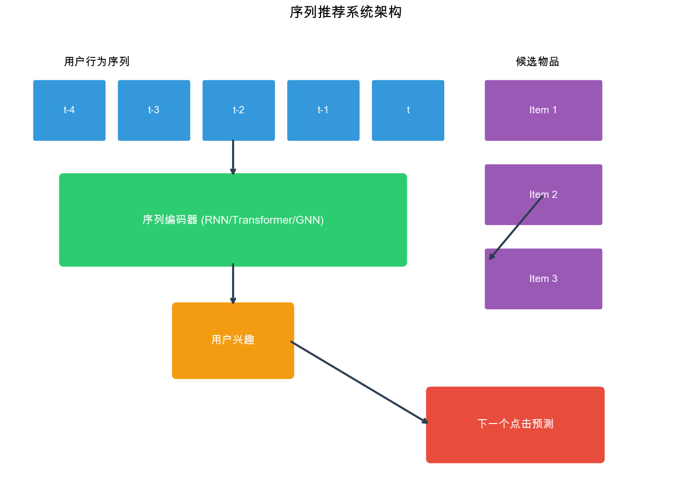
Sequential recommendation is a paradigm that models user preferences by analyzing the temporal order of their interactions with items. Unlike traditional collaborative filtering that treats interactions as independent, sequential recommendation recognizes that user preferences evolve over time and that the sequence of interactions contains valuable signals for prediction.

Formally, given a user \(u\)with an interaction sequence\(S_u = [i_1, i_2, \dots, i_t]\)where\(i_j\)is the\(j\)-th item the user interacted with, sequential recommendation aims to predict the next item\(i_{t+1}\)the user will interact with:\[P(i_{t+1} | S_u) = P(i_{t+1} | i_1, i_2, \dots, i_t)\]The key insight is that the order matters: the probability of interacting with item\(i_{t+1}\)depends not just on the set of items seen before, but on their specific ordering.

Why Sequential Recommendation Matters

Temporal Dynamics: User preferences change over time. A user who watched action movies last month might now prefer documentaries. Sequential models capture these shifts.

Context Dependency: The next item depends on recent context. After watching a movie trailer, you're more likely to watch the full movie than a random video.

Session Patterns: In e-commerce, users often browse within sessions. Sequential models can capture session-level patterns (e.g., "users who view laptops often view laptop bags next").

Cold Start Mitigation: For new users with limited history, sequential models can leverage the sequence structure even with few interactions.

Sequential vs. Traditional Recommendation

Aspect	Traditional CF	Sequential Recommendation
Input	Set of user-item interactions	Ordered sequence of interactions
Temporal Modeling	Ignores order	Explicitly models order
Prediction	\(P(i \| u)\)	\(P(i_{t+1} \| S_u)\)
Use Case	Long-term preferences	Next-item prediction
Example	"Users like you also liked..."	"Based on your recent viewing..."

Types of Sequential Recommendation

1. User-based Sequential Recommendation: Models the entire user history as a sequence. Suitable for long-term preference modeling.

2. Session-based Recommendation: Models short sessions independently. Each session is a sequence, and sessions are treated independently. Ideal for anonymous users or short-term patterns.

3. Hybrid Approaches: Combine user-level and session-level signals for better prediction.

Markov Chain Models

First-Order Markov Chains

The simplest sequential model is a first-order Markov chain, which assumes that the next item depends only on the current item:\[P(i_{t+1} | i_1, i_2, \dots, i_t) = P(i_{t+1} | i_t)\]This is a strong independence assumption: it ignores all history except the most recent item.

Transition Matrix: We learn a transition matrix\(M \in \mathbb{R}^{|I| \times |I|}\)where\(M_{ij} = P(j | i)\)represents the probability of transitioning from item\(i\)to item\(j\).

Given a sequence\(S = [i_1, i_2, \dots, i_T]\), we estimate:\[M_{ij} = \frac{\text{count}(i \rightarrow j)}{\text{count}(i)}\]where\(\text{count}(i \rightarrow j)\)is the number of times item\(j\)follows item\(i\)in all sequences, and\(\text{count}(i)\)is the number of times item\(i\)appears (except as the last item).

Higher-Order Markov Chains

A \(k\)-th order Markov chain assumes the next item depends on the last\(k\)items:\[P(i_{t+1} | i_1, i_2, \dots, i_t) = P(i_{t+1} | i_{t-k+1}, \dots, i_t)\]Higher-order models capture more context but suffer from data sparsity: the number of possible\(k\)-grams grows exponentially with\(k\).

Implementation: Markov Chain Recommender

import numpy as np
from collections import defaultdict
from typing import List, Dict

class MarkovChainRecommender:
    """
    First-order Markov chain for sequential recommendation.
    """
    def __init__(self, order: int = 1):
        self.order = order
        self.transition_counts = defaultdict(lambda: defaultdict(int))
        self.item_counts = defaultdict(int)
        self.items = set()
    
    def fit(self, sequences: List[List[int]]):
        """
        Learn transition probabilities from sequences.
        
        Args:
            sequences: List of interaction sequences, each is [item_id1, item_id2, ...]
        """
        for sequence in sequences:
            self.items.update(sequence)
            for i in range(len(sequence) - self.order):
                # Get the context (last k items)
                context = tuple(sequence[i:i+self.order])
                next_item = sequence[i + self.order]
                
                self.transition_counts[context][next_item] += 1
                self.item_counts[context] += 1
    
    def predict_next(self, sequence: List[int], top_k: int = 10) -> List[tuple]:
        """
        Predict next items given a sequence.
        
        Args:
            sequence: Current interaction sequence
            top_k: Number of top items to return
            
        Returns:
            List of (item_id, probability) tuples
        """
        if len(sequence) < self.order:
            # Not enough history, return most popular items
            return self._get_most_popular(top_k)
        
        context = tuple(sequence[-self.order:])
        
        if context not in self.transition_counts:
            return self._get_most_popular(top_k)
        
        # Get transition probabilities
        transitions = self.transition_counts[context]
        total = self.item_counts[context]
        
        probs = [(item, count / total) 
                 for item, count in transitions.items()]
        probs.sort(key=lambda x: x[1], reverse=True)
        
        return probs[:top_k]
    
    def _get_most_popular(self, top_k: int) -> List[tuple]:
        """Fallback to most popular items."""
        # Simple implementation: return random items
        # In practice, you'd maintain global item popularity
        return [(item, 0.0) for item in list(self.items)[:top_k]]

# Example usage
if __name__ == "__main__":
    # Sample sequences: users browsing products
    sequences = [
        [1, 2, 3, 4],  # User 1: laptop -> mouse -> keyboard -> monitor
        [1, 2, 5],     # User 2: laptop -> mouse -> mousepad
        [2, 3, 4],     # User 3: mouse -> keyboard -> monitor
        [1, 6, 7],     # User 4: laptop -> charger -> bag
    ]
    
    model = MarkovChainRecommender(order=1)
    model.fit(sequences)
    
    # Predict next item for sequence [1, 2]
    predictions = model.predict_next([1, 2], top_k=5)
    print("Predictions for sequence [1, 2]:")
    for item, prob in predictions:
        print(f"  Item {item}: {prob:.3f}")

Limitations of Markov Chains

Data Sparsity: For large item catalogs, most transitions are never observed. Smoothing techniques (e.g., Laplace smoothing) help but don't fully solve the problem.

Limited Context: Even higher-order Markov chains only consider a fixed window of history, missing long-term dependencies.

No Generalization: Markov chains don't generalize across similar items. If items\(A\)and\(B\)are similar, a Markov chain doesn't leverage this similarity.

GRU4Rec: RNN-Based Sequential Recommendation

Architecture Overview

GRU4Rec (GRU for Recommendation), introduced by Hidasi et al. in 2015, was one of the first deep learning models for session-based recommendation. It uses Gated Recurrent Units (GRUs) to model sequential patterns in user sessions.

Key Innovation: Instead of treating sessions as bags of items, GRU4Rec processes items sequentially, allowing the model to learn how user preferences evolve within a session.

GRU Architecture

A GRU cell maintains a hidden state\(h_t\)that summarizes the history up to time\(t\). Given input\(x_t\)(embedding of item\(i_t\)) and previous hidden state\(h_{t-1}\), the GRU computes:

Reset Gate:\[r_t = \sigma(W_r x_t + U_r h_{t-1} + b_r)\]

Update Gate:\[z_t = \sigma(W_z x_t + U_z h_{t-1} + b_z)\]

Candidate Activation:\[\tilde{h}_t = \tanh(W_h x_t + U_h (r_t \odot h_{t-1}) + b_h)\]

Hidden State:\[h_t = (1 - z_t) \odot h_{t-1} + z_t \odot \tilde{h}_t\]where\(\sigma\)is the sigmoid function,\(\odot\)is element-wise multiplication, and\(W_r, U_r, W_z, U_z, W_h, U_h\)are learnable weight matrices.

GRU4Rec Model Structure

1. Embedding Layer: Maps item IDs to dense vectors:\(\mathbf{e}_t = \text{Embedding}(i_t) \in \mathbb{R}^d\)

2. GRU Layer: Processes the sequence:\(h_t = \text{GRU}(\mathbf{e}_t, h_{t-1})\)

3. Output Layer: Predicts next item probabilities:\[\hat{y}_t = \text{softmax}(W_o h_t + b_o)\]

4. Loss Function: Uses ranking loss (BPR or TOP1) instead of cross-entropy to handle implicit feedback.

Implementation: GRU4Rec

import torch
import torch.nn as nn
import torch.nn.functional as F
from torch.utils.data import Dataset, DataLoader
import numpy as np

class GRU4Rec(nn.Module):
    """
    GRU4Rec model for session-based recommendation.
    """
    def __init__(self, num_items: int, embedding_dim: int = 128, 
                 hidden_dim: int = 128, num_layers: int = 1, 
                 dropout: float = 0.25):
        super(GRU4Rec, self).__init__()
        self.num_items = num_items
        self.embedding_dim = embedding_dim
        self.hidden_dim = hidden_dim
        
        # Embedding layer
        self.item_embedding = nn.Embedding(num_items + 1, embedding_dim, padding_idx=0)
        
        # GRU layer
        self.gru = nn.GRU(
            input_size=embedding_dim,
            hidden_size=hidden_dim,
            num_layers=num_layers,
            batch_first=True,
            dropout=dropout if num_layers > 1 else 0
        )
        
        # Output layer
        self.output = nn.Linear(hidden_dim, num_items + 1)
        
        # Dropout
        self.dropout = nn.Dropout(dropout)
        
        self._init_weights()
    
    def _init_weights(self):
        """Initialize weights."""
        nn.init.normal_(self.item_embedding.weight, mean=0, std=0.01)
        nn.init.xavier_uniform_(self.output.weight)
        nn.init.zeros_(self.output.bias)
    
    def forward(self, sequences, hidden=None):
        """
        Forward pass.
        
        Args:
            sequences: (batch_size, seq_len) tensor of item indices
            hidden: Initial hidden state
            
        Returns:
            logits: (batch_size, seq_len, num_items+1) prediction logits
            hidden: Final hidden state
        """
        # Embed items
        embedded = self.item_embedding(sequences)  # (batch, seq_len, emb_dim)
        embedded = self.dropout(embedded)
        
        # Process through GRU
        gru_out, hidden = self.gru(embedded, hidden)  # (batch, seq_len, hidden_dim)
        gru_out = self.dropout(gru_out)
        
        # Predict next items
        logits = self.output(gru_out)  # (batch, seq_len, num_items+1)
        
        return logits, hidden
    
    def predict_next(self, sequence, top_k=10):
        """
        Predict next items for a sequence.
        
        Args:
            sequence: List of item indices
            top_k: Number of top items to return
            
        Returns:
            List of (item_id, score) tuples
        """
        self.eval()
        with torch.no_grad():
            # Convert to tensor
            seq_tensor = torch.LongTensor([sequence]).to(next(self.parameters()).device)
            
            # Forward pass
            logits, _ = self.forward(seq_tensor)
            
            # Get prediction for last position
            last_logits = logits[0, -1, :]  # (num_items+1,)
            
            # Get top-k
            top_scores, top_indices = torch.topk(last_logits, k=min(top_k, self.num_items))
            
            return [(idx.item(), score.item()) 
                    for idx, score in zip(top_indices, top_scores)]

class SessionDataset(Dataset):
    """Dataset for session-based recommendation."""
    def __init__(self, sessions, max_len=20):
        self.sessions = sessions
        self.max_len = max_len
    
    def __len__(self):
        return len(self.sessions)
    
    def __getitem__(self, idx):
        session = self.sessions[idx]
        
        # Pad or truncate to max_len
        if len(session) > self.max_len:
            session = session[-self.max_len:]
        else:
            session = [0] * (self.max_len - len(session)) + session
        
        # Input is all but last item, target is all but first item
        input_seq = torch.LongTensor(session[:-1])
        target_seq = torch.LongTensor(session[1:])
        
        return input_seq, target_seq

def train_gru4rec(model, train_loader, num_epochs=10, lr=0.001, device='cpu'):
    """Train GRU4Rec model."""
    optimizer = torch.optim.Adam(model.parameters(), lr=lr)
    criterion = nn.CrossEntropyLoss(ignore_index=0)  # Ignore padding
    
    model.to(device)
    model.train()
    
    for epoch in range(num_epochs):
        total_loss = 0
        for batch_inputs, batch_targets in train_loader:
            batch_inputs = batch_inputs.to(device)
            batch_targets = batch_targets.to(device)
            
            optimizer.zero_grad()
            
            # Forward pass
            logits, _ = model(batch_inputs)
            
            # Reshape for loss computation
            logits = logits.reshape(-1, logits.size(-1))
            targets = batch_targets.reshape(-1)
            
            # Compute loss
            loss = criterion(logits, targets)
            
            # Backward pass
            loss.backward()
            optimizer.step()
            
            total_loss += loss.item()
        
        print(f"Epoch {epoch+1}/{num_epochs}, Loss: {total_loss/len(train_loader):.4f}")

# Example usage
if __name__ == "__main__":
    # Sample sessions
    sessions = [
        [1, 2, 3, 4],
        [5, 6, 7],
        [1, 8, 9, 10],
        [2, 3, 11],
    ]
    
    num_items = max(max(s) for s in sessions)
    
    # Create dataset
    dataset = SessionDataset(sessions, max_len=10)
    train_loader = DataLoader(dataset, batch_size=2, shuffle=True)
    
    # Create model
    model = GRU4Rec(num_items=num_items, embedding_dim=64, hidden_dim=64)
    
    # Train
    train_gru4rec(model, train_loader, num_epochs=5)
    
    # Predict
    predictions = model.predict_next([1, 2, 3], top_k=5)
    print("\nPredictions for sequence [1, 2, 3]:")
    for item, score in predictions:
        print(f"  Item {item}: {score:.3f}")

Advantages and Limitations

Advantages: - Captures sequential dependencies - Handles variable-length sequences - Can model long-term dependencies (with sufficient capacity)

Limitations: - Sequential processing is slow (can't parallelize) - Difficulty capturing very long dependencies - Fixed context window in practice

Caser: Convolutional Sequence Embedding

Motivation

Caser (Convolutional Sequence Embedding), introduced by Tang and Wang in 2018, applies convolutional neural networks to sequential recommendation. Unlike RNNs that process sequences sequentially, CNNs can process sequences in parallel and capture both local and global patterns through different filter sizes.

Architecture

Caser models sequences at two levels:

1. Point-level: Captures point-wise patterns (individual items)
2. Union-level: Captures union patterns (combinations of items)

The model uses horizontal and vertical convolutional filters:

Horizontal Filters: Slide over the sequence to capture union-level patterns of different lengths.

Vertical Filters: Operate on the embedding dimension to capture point-level patterns.

Mathematical Formulation

Given a sequence\(S = [i_1, i_2, \dots, i_t]\)and embeddings\(\mathbf{E} = [\mathbf{e}_1, \mathbf{e}_2, \dots, \mathbf{e}_t] \in \mathbb{R}^{t \times d}\), Caser applies:

Horizontal Convolution: For filter size\(h\):\[\mathbf{c}_h = \text{ReLU}(\text{Conv1D}_h(\mathbf{E}))\]

Vertical Convolution:\[\mathbf{c}_v = \text{ReLU}(\text{Conv2D}(\mathbf{E}))\]The outputs are concatenated and passed through fully connected layers to predict the next item.

Implementation: Caser

import torch
import torch.nn as nn
import torch.nn.functional as F

class Caser(nn.Module):
    """
    Caser model for sequential recommendation using CNNs.
    """
    def __init__(self, num_items: int, embedding_dim: int = 50, 
                 max_len: int = 50, num_horizon_filters: int = 16,
                 num_vertical_filters: int = 8, horizon_filter_sizes: list = [2, 3, 4]):
        super(Caser, self).__init__()
        self.num_items = num_items
        self.embedding_dim = embedding_dim
        self.max_len = max_len
        
        # Item embedding
        self.item_embedding = nn.Embedding(num_items + 1, embedding_dim, padding_idx=0)
        
        # Horizontal (union-level) convolutional filters
        self.horizon_convs = nn.ModuleList([
            nn.Conv2d(1, num_horizon_filters, (h, embedding_dim))
            for h in horizon_filter_sizes
        ])
        
        # Vertical (point-level) convolutional filter
        self.vertical_conv = nn.Conv2d(1, num_vertical_filters, (max_len, 1))
        
        # Fully connected layers
        total_dim = num_horizon_filters * len(horizon_filter_sizes) + num_vertical_filters
        self.fc1 = nn.Linear(total_dim, embedding_dim)
        self.fc2 = nn.Linear(embedding_dim, num_items + 1)
        
        self.dropout = nn.Dropout(0.5)
        self._init_weights()
    
    def _init_weights(self):
        """Initialize weights."""
        nn.init.normal_(self.item_embedding.weight, mean=0, std=0.01)
        nn.init.xavier_uniform_(self.fc1.weight)
        nn.init.xavier_uniform_(self.fc2.weight)
    
    def forward(self, sequences):
        """
        Forward pass.
        
        Args:
            sequences: (batch_size, seq_len) tensor of item indices
            
        Returns:
            logits: (batch_size, num_items+1) prediction logits
        """
        batch_size = sequences.size(0)
        
        # Embed items
        embedded = self.item_embedding(sequences)  # (batch, seq_len, emb_dim)
        
        # Add channel dimension for convolution
        embedded = embedded.unsqueeze(1)  # (batch, 1, seq_len, emb_dim)
        
        # Horizontal convolutions (union-level)
        horizon_outs = []
        for conv in self.horizon_convs:
            # Conv2d: (batch, 1, seq_len, emb_dim) -> (batch, num_filters, out_h, out_w)
            conv_out = F.relu(conv(embedded))  # (batch, num_filters, out_h, 1)
            # Max pooling over sequence dimension
            pooled = F.max_pool2d(conv_out, kernel_size=(conv_out.size(2), 1))
            # Flatten
            horizon_outs.append(pooled.squeeze(-1).squeeze(-1))  # (batch, num_filters)
        
        horizon_out = torch.cat(horizon_outs, dim=1)  # (batch, total_horizon_filters)
        
        # Vertical convolution (point-level)
        vertical_out = F.relu(self.vertical_conv(embedded))  # (batch, num_filters, 1, emb_dim)
        vertical_out = vertical_out.squeeze(2).squeeze(2)  # (batch, num_filters)
        
        # Concatenate
        combined = torch.cat([horizon_out, vertical_out], dim=1)  # (batch, total_dim)
        
        # Fully connected layers
        out = self.dropout(F.relu(self.fc1(combined)))
        logits = self.fc2(out)  # (batch, num_items+1)
        
        return logits
    
    def predict_next(self, sequence, top_k=10):
        """Predict next items."""
        self.eval()
        with torch.no_grad():
            # Pad sequence to max_len
            if len(sequence) > self.max_len:
                sequence = sequence[-self.max_len:]
            else:
                sequence = [0] * (self.max_len - len(sequence)) + sequence
            
            seq_tensor = torch.LongTensor([sequence]).to(next(self.parameters()).device)
            
            logits = self.forward(seq_tensor)
            top_scores, top_indices = torch.topk(logits[0], k=min(top_k, self.num_items))
            
            return [(idx.item(), score.item()) 
                    for idx, score in zip(top_indices, top_scores)]

# Example usage
if __name__ == "__main__":
    num_items = 1000
    model = Caser(num_items=num_items, embedding_dim=50, max_len=50)
    
    # Sample sequence
    sequence = [1, 2, 3, 4, 5]
    predictions = model.predict_next(sequence, top_k=5)
    print("Caser predictions:")
    for item, score in predictions:
        print(f"  Item {item}: {score:.3f}")

Advantages of Caser

• Parallel Processing: CNNs process sequences in parallel, faster than RNNs
• Multi-scale Patterns: Different filter sizes capture patterns at different scales
• Local Patterns: Excellent at capturing local sequential patterns

SASRec: Self-Attention for Sequential Recommendation

Transformer Architecture

SASRec (Self-Attention Sequential Recommendation), introduced by Kang and McAuley in 2018, adapts the Transformer architecture for sequential recommendation. It uses self-attention mechanisms to model long-range dependencies without the sequential processing bottleneck of RNNs.

Key Components

1. Self-Attention Mechanism: Allows each position to attend to all previous positions:\[\text{Attention}(Q, K, V) = \text{softmax}\left(\frac{QK^T}{\sqrt{d_k }}\right)V\]where\(Q\),\(K\),\(V\)are query, key, and value matrices derived from item embeddings.

2. Positional Encoding: Since Transformers have no inherent notion of order, positional encodings are added to embeddings:$\(PE_{(pos, 2i)} = \sin(pos / 10000^{2i/d})\) $

\[PE_{(pos, 2i+1)} = \cos(pos / 10000^{2i/d})\]

3. Point-wise Feed-Forward Networks: Applied after attention for non-linearity.

4. Layer Normalization and Residual Connections: Enable training of deep networks.

Implementation: SASRec

import torch
import torch.nn as nn
import torch.nn.functional as F
import math

class PositionalEncoding(nn.Module):
    """Positional encoding for sequences."""
    def __init__(self, d_model, max_len=5000):
        super(PositionalEncoding, self).__init__()
        
        pe = torch.zeros(max_len, d_model)
        position = torch.arange(0, max_len, dtype=torch.float).unsqueeze(1)
        div_term = torch.exp(torch.arange(0, d_model, 2).float() * 
                            (-math.log(10000.0) / d_model))
        pe[:, 0::2] = torch.sin(position * div_term)
        pe[:, 1::2] = torch.cos(position * div_term)
        pe = pe.unsqueeze(0)  # (1, max_len, d_model)
        self.register_buffer('pe', pe)
    
    def forward(self, x):
        """
        Args:
            x: (batch_size, seq_len, d_model)
        """
        return x + self.pe[:, :x.size(1), :]

class MultiHeadAttention(nn.Module):
    """Multi-head self-attention."""
    def __init__(self, d_model, num_heads, dropout=0.1):
        super(MultiHeadAttention, self).__init__()
        assert d_model % num_heads == 0
        
        self.d_model = d_model
        self.num_heads = num_heads
        self.d_k = d_model // num_heads
        
        self.W_q = nn.Linear(d_model, d_model)
        self.W_k = nn.Linear(d_model, d_model)
        self.W_v = nn.Linear(d_model, d_model)
        self.W_o = nn.Linear(d_model, d_model)
        
        self.dropout = nn.Dropout(dropout)
    
    def forward(self, query, key, value, mask=None):
        """
        Args:
            query, key, value: (batch_size, seq_len, d_model)
            mask: (batch_size, seq_len, seq_len) attention mask
        """
        batch_size = query.size(0)
        
        # Linear projections and reshape for multi-head
        Q = self.W_q(query).view(batch_size, -1, self.num_heads, self.d_k).transpose(1, 2)
        K = self.W_k(key).view(batch_size, -1, self.num_heads, self.d_k).transpose(1, 2)
        V = self.W_v(value).view(batch_size, -1, self.num_heads, self.d_k).transpose(1, 2)
        
        # Scaled dot-product attention
        scores = torch.matmul(Q, K.transpose(-2, -1)) / math.sqrt(self.d_k)
        
        # Apply mask (causal mask for sequential recommendation)
        if mask is not None:
            scores = scores.masked_fill(mask == 0, -1e9)
        
        attn_weights = F.softmax(scores, dim=-1)
        attn_weights = self.dropout(attn_weights)
        
        # Apply attention to values
        context = torch.matmul(attn_weights, V)
        
        # Concatenate heads
        context = context.transpose(1, 2).contiguous().view(
            batch_size, -1, self.d_model
        )
        
        output = self.W_o(context)
        return output, attn_weights

class TransformerBlock(nn.Module):
    """Transformer block with self-attention and feed-forward."""
    def __init__(self, d_model, num_heads, d_ff, dropout=0.1):
        super(TransformerBlock, self).__init__()
        
        self.attention = MultiHeadAttention(d_model, num_heads, dropout)
        self.norm1 = nn.LayerNorm(d_model)
        self.norm2 = nn.LayerNorm(d_model)
        
        self.feed_forward = nn.Sequential(
            nn.Linear(d_model, d_ff),
            nn.ReLU(),
            nn.Dropout(dropout),
            nn.Linear(d_ff, d_model),
            nn.Dropout(dropout)
        )
    
    def forward(self, x, mask=None):
        # Self-attention with residual
        attn_out, _ = self.attention(x, x, x, mask)
        x = self.norm1(x + attn_out)
        
        # Feed-forward with residual
        ff_out = self.feed_forward(x)
        x = self.norm2(x + ff_out)
        
        return x

class SASRec(nn.Module):
    """
    SASRec: Self-Attention Sequential Recommendation.
    """
    def __init__(self, num_items: int, d_model: int = 128, num_heads: int = 2,
                 num_layers: int = 2, d_ff: int = 256, max_len: int = 50,
                 dropout: float = 0.1):
        super(SASRec, self).__init__()
        self.num_items = num_items
        self.d_model = d_model
        self.max_len = max_len
        
        # Item embedding
        self.item_embedding = nn.Embedding(num_items + 1, d_model, padding_idx=0)
        
        # Positional encoding
        self.pos_encoding = PositionalEncoding(d_model, max_len)
        
        # Transformer blocks
        self.transformer_blocks = nn.ModuleList([
            TransformerBlock(d_model, num_heads, d_ff, dropout)
            for _ in range(num_layers)
        ])
        
        # Dropout
        self.dropout = nn.Dropout(dropout)
        
        # Output layer
        self.output = nn.Linear(d_model, num_items + 1)
        
        self._init_weights()
    
    def _init_weights(self):
        """Initialize weights."""
        nn.init.normal_(self.item_embedding.weight, mean=0, std=0.01)
        nn.init.xavier_uniform_(self.output.weight)
        nn.init.zeros_(self.output.bias)
    
    def _generate_mask(self, sequences):
        """
        Generate causal mask for sequences.
        
        Args:
            sequences: (batch_size, seq_len)
            
        Returns:
            mask: (batch_size, seq_len, seq_len)
        """
        batch_size, seq_len = sequences.size()
        # Causal mask: can attend to current and previous positions
        mask = torch.tril(torch.ones(seq_len, seq_len)).unsqueeze(0).repeat(batch_size, 1, 1)
        # Mask out padding positions
        padding_mask = (sequences != 0).unsqueeze(1).unsqueeze(2)
        mask = mask * padding_mask.float()
        return mask.to(sequences.device)
    
    def forward(self, sequences):
        """
        Forward pass.
        
        Args:
            sequences: (batch_size, seq_len) tensor of item indices
            
        Returns:
            logits: (batch_size, seq_len, num_items+1) prediction logits
        """
        # Embed items
        embedded = self.item_embedding(sequences) * math.sqrt(self.d_model)
        
        # Add positional encoding
        embedded = self.pos_encoding(embedded)
        embedded = self.dropout(embedded)
        
        # Generate mask
        mask = self._generate_mask(sequences)
        
        # Pass through transformer blocks
        x = embedded
        for transformer in self.transformer_blocks:
            x = transformer(x, mask)
        
        # Predict next items
        logits = self.output(x)  # (batch, seq_len, num_items+1)
        
        return logits
    
    def predict_next(self, sequence, top_k=10):
        """Predict next items."""
        self.eval()
        with torch.no_grad():
            # Pad or truncate sequence
            if len(sequence) > self.max_len:
                sequence = sequence[-self.max_len:]
            else:
                sequence = [0] * (self.max_len - len(sequence)) + sequence
            
            seq_tensor = torch.LongTensor([sequence]).to(next(self.parameters()).device)
            
            logits = self.forward(seq_tensor)
            # Get prediction for last position
            last_logits = logits[0, -1, :]
            
            top_scores, top_indices = torch.topk(last_logits, k=min(top_k, self.num_items))
            
            return [(idx.item(), score.item()) 
                    for idx, score in zip(top_indices, top_scores)]

# Example usage
if __name__ == "__main__":
    num_items = 1000
    model = SASRec(num_items=num_items, d_model=128, num_heads=2, num_layers=2)
    
    sequence = [1, 2, 3, 4, 5]
    predictions = model.predict_next(sequence, top_k=5)
    print("SASRec predictions:")
    for item, score in predictions:
        print(f"  Item {item}: {score:.3f}")

Advantages of SASRec

• Long-range Dependencies: Self-attention can model dependencies across the entire sequence
• Parallel Processing: All positions processed simultaneously
• Interpretability: Attention weights show which items influence predictions
• Scalability: Efficient for long sequences

BERT4Rec: Bidirectional Encoder for Sequential Recommendation

Motivation

BERT4Rec, introduced by Sun et al. in 2019, adapts BERT (Bidirectional Encoder Representations from Transformers) for sequential recommendation. Unlike SASRec which uses causal (unidirectional) attention, BERT4Rec uses bidirectional attention, allowing each position to attend to both past and future items.

Key Innovation: Cloze Task

BERT4Rec trains using a cloze task (masked language modeling): randomly mask some items in the sequence and predict them from context. This bidirectional training allows the model to leverage both past and future context.

Architecture Differences from SASRec

1. Bidirectional Attention: No causal mask; each position can attend to all positions
2. Masked Training: Randomly mask items during training
3. Two-stage Training: Pre-training on large datasets, then fine-tuning

Implementation: BERT4Rec

import torch
import torch.nn as nn
import torch.nn.functional as F
import math
import random

class BERT4Rec(nn.Module):
    """
    BERT4Rec: Bidirectional Encoder for Sequential Recommendation.
    """
    def __init__(self, num_items: int, d_model: int = 128, num_heads: int = 2,
                 num_layers: int = 2, d_ff: int = 256, max_len: int = 50,
                 dropout: float = 0.1, mask_prob: float = 0.15):
        super(BERT4Rec, self).__init__()
        self.num_items = num_items
        self.d_model = d_model
        self.max_len = max_len
        self.mask_prob = mask_prob
        
        # Special tokens: [PAD]=0, [MASK]=num_items+1
        self.mask_token = num_items + 1
        
        # Item embedding (including mask token)
        self.item_embedding = nn.Embedding(num_items + 2, d_model, padding_idx=0)
        
        # Positional encoding
        self.pos_encoding = PositionalEncoding(d_model, max_len)
        
        # Transformer blocks (bidirectional, no causal mask)
        self.transformer_blocks = nn.ModuleList([
            TransformerBlock(d_model, num_heads, d_ff, dropout)
            for _ in range(num_layers)
        ])
        
        self.dropout = nn.Dropout(dropout)
        
        # Output layer
        self.output = nn.Linear(d_model, num_items + 1)
        
        self._init_weights()
    
    def _init_weights(self):
        """Initialize weights."""
        nn.init.normal_(self.item_embedding.weight, mean=0, std=0.01)
        nn.init.xavier_uniform_(self.output.weight)
        nn.init.zeros_(self.output.bias)
    
    def _generate_mask(self, sequences):
        """
        Generate padding mask (no causal mask for bidirectional).
        
        Args:
            sequences: (batch_size, seq_len)
            
        Returns:
            mask: (batch_size, seq_len, seq_len)
        """
        batch_size, seq_len = sequences.size()
        # All positions can attend to all positions (except padding)
        mask = (sequences != 0).unsqueeze(1).unsqueeze(2).float()
        mask = mask.repeat(1, seq_len, seq_len)
        return mask.to(sequences.device)
    
    def _mask_sequence(self, sequences):
        """
        Randomly mask items for cloze task training.
        
        Args:
            sequences: (batch_size, seq_len)
            
        Returns:
            masked_sequences: (batch_size, seq_len) with some items masked
            masked_positions: (batch_size, seq_len) boolean mask
        """
        masked_sequences = sequences.clone()
        masked_positions = torch.zeros_like(sequences, dtype=torch.bool)
        
        for i in range(sequences.size(0)):
            for j in range(sequences.size(1)):
                if sequences[i, j] != 0:  # Not padding
                    if random.random() < self.mask_prob:
                        masked_positions[i, j] = True
                        # 80% mask, 10% random, 10% unchanged
                        rand = random.random()
                        if rand < 0.8:
                            masked_sequences[i, j] = self.mask_token
                        elif rand < 0.9:
                            masked_sequences[i, j] = random.randint(1, self.num_items)
                        # else: keep original
        
        return masked_sequences, masked_positions
    
    def forward(self, sequences, training=True):
        """
        Forward pass.
        
        Args:
            sequences: (batch_size, seq_len) tensor of item indices
            training: If True, apply masking for cloze task
            
        Returns:
            logits: (batch_size, seq_len, num_items+1) prediction logits
            masked_positions: (batch_size, seq_len) positions that were masked
        """
        if training:
            sequences, masked_positions = self._mask_sequence(sequences)
        else:
            masked_positions = torch.zeros_like(sequences, dtype=torch.bool)
        
        # Embed items
        embedded = self.item_embedding(sequences) * math.sqrt(self.d_model)
        
        # Add positional encoding
        embedded = self.pos_encoding(embedded)
        embedded = self.dropout(embedded)
        
        # Generate padding mask (bidirectional attention)
        mask = self._generate_mask(sequences)
        
        # Pass through transformer blocks
        x = embedded
        for transformer in self.transformer_blocks:
            x = transformer(x, mask)
        
        # Predict items
        logits = self.output(x)  # (batch, seq_len, num_items+1)
        
        return logits, masked_positions
    
    def predict_next(self, sequence, top_k=10):
        """
        Predict next items. For inference, we append a [MASK] token.
        """
        self.eval()
        with torch.no_grad():
            # Append mask token
            if len(sequence) >= self.max_len:
                sequence = sequence[-(self.max_len-1):] + [self.mask_token]
            else:
                sequence = sequence + [self.mask_token]
                # Pad to max_len
                sequence = [0] * (self.max_len - len(sequence)) + sequence
            
            seq_tensor = torch.LongTensor([sequence]).to(next(self.parameters()).device)
            
            logits, _ = self.forward(seq_tensor, training=False)
            # Get prediction for mask token position
            mask_pos = sequence.index(self.mask_token)
            mask_logits = logits[0, mask_pos, :]
            
            top_scores, top_indices = torch.topk(mask_logits, k=min(top_k, self.num_items))
            
            return [(idx.item(), score.item()) 
                    for idx, score in zip(top_indices, top_scores)]

# Example usage
if __name__ == "__main__":
    num_items = 1000
    model = BERT4Rec(num_items=num_items, d_model=128, num_heads=2, num_layers=2)
    
    sequence = [1, 2, 3, 4, 5]
    predictions = model.predict_next(sequence, top_k=5)
    print("BERT4Rec predictions:")
    for item, score in predictions:
        print(f"  Item {item}: {score:.3f}")

Advantages of BERT4Rec

• Bidirectional Context: Leverages both past and future information
• Better Representations: Pre-training on large datasets learns rich item representations
• Robustness: Masked training makes the model more robust to missing items

Limitations

• Inference Complexity: Requires masking during inference, which is less intuitive than autoregressive prediction
• Training Complexity: Two-stage training (pre-training + fine-tuning) is more complex

BST: Behavior Sequence Transformer

Introduction

BST (Behavior Sequence Transformer), introduced by Chen et al. in 2019, extends the Transformer architecture to incorporate rich feature information beyond item IDs. It's designed for e-commerce recommendation where user behaviors include clicks, views, purchases, and various item features.

Key Features

1. Multi-field Features: Incorporates item features (category, brand, price), user features, and context features
2. Behavior Sequence: Models sequences of user behaviors (not just items)
3. Feature Interaction: Uses point-wise and element-wise feature interactions

Architecture

BST consists of:

1. Embedding Layer: Embeds item IDs and all feature fields
2. Positional Encoding: Adds positional information
3. Transformer Layers: Self-attention over behavior sequences
4. MLP Layers: Final prediction with feature interactions

Implementation: BST

import torch
import torch.nn as nn
import torch.nn.functional as F

class FeatureEmbedding(nn.Module):
    """Embedding layer for multi-field features."""
    def __init__(self, feature_dims, embedding_dim):
        """
        Args:
            feature_dims: Dict mapping feature name to vocabulary size
            embedding_dim: Embedding dimension
        """
        super(FeatureEmbedding, self).__init__()
        self.embedding_dim = embedding_dim
        self.embeddings = nn.ModuleDict({
            name: nn.Embedding(dim + 1, embedding_dim, padding_idx=0)
            for name, dim in feature_dims.items()
        })
    
    def forward(self, features):
        """
        Args:
            features: Dict of (batch_size, seq_len) tensors
            
        Returns:
            embedded: (batch_size, seq_len, num_fields * embedding_dim)
        """
        embedded_list = []
        for name, tensor in features.items():
            embedded_list.append(self.embeddings[name](tensor))
        
        # Concatenate all feature embeddings
        embedded = torch.cat(embedded_list, dim=-1)
        return embedded

class BST(nn.Module):
    """
    BST: Behavior Sequence Transformer for E-commerce Recommendation.
    """
    def __init__(self, item_vocab_size: int, feature_dims: dict, embedding_dim: int = 64,
                 num_heads: int = 2, num_layers: int = 2, d_ff: int = 256,
                 max_len: int = 50, dropout: float = 0.1):
        super(BST, self).__init__()
        self.item_vocab_size = item_vocab_size
        self.embedding_dim = embedding_dim
        self.max_len = max_len
        self.num_fields = len(feature_dims) + 1  # +1 for item_id
        
        # Item embedding
        self.item_embedding = nn.Embedding(item_vocab_size + 1, embedding_dim, padding_idx=0)
        
        # Feature embeddings
        self.feature_embedding = FeatureEmbedding(feature_dims, embedding_dim)
        
        # Total embedding dimension
        total_emb_dim = embedding_dim + embedding_dim * len(feature_dims)
        
        # Positional encoding
        self.pos_encoding = PositionalEncoding(total_emb_dim, max_len)
        
        # Transformer blocks
        self.transformer_blocks = nn.ModuleList([
            TransformerBlock(total_emb_dim, num_heads, d_ff, dropout)
            for _ in range(num_layers)
        ])
        
        self.dropout = nn.Dropout(dropout)
        
        # MLP for final prediction
        self.mlp = nn.Sequential(
            nn.Linear(total_emb_dim, d_ff),
            nn.ReLU(),
            nn.Dropout(dropout),
            nn.Linear(d_ff, d_ff // 2),
            nn.ReLU(),
            nn.Dropout(dropout),
            nn.Linear(d_ff // 2, 1)
        )
        
        self._init_weights()
    
    def _init_weights(self):
        """Initialize weights."""
        nn.init.normal_(self.item_embedding.weight, mean=0, std=0.01)
        for emb in self.feature_embedding.embeddings.values():
            nn.init.normal_(emb.weight, mean=0, std=0.01)
    
    def _generate_mask(self, sequences):
        """Generate causal mask."""
        batch_size, seq_len = sequences.size()
        mask = torch.tril(torch.ones(seq_len, seq_len)).unsqueeze(0).repeat(batch_size, 1, 1)
        padding_mask = (sequences != 0).unsqueeze(1).unsqueeze(2)
        mask = mask * padding_mask.float()
        return mask.to(sequences.device)
    
    def forward(self, item_ids, features):
        """
        Forward pass.
        
        Args:
            item_ids: (batch_size, seq_len) item IDs
            features: Dict of (batch_size, seq_len) feature tensors
            
        Returns:
            scores: (batch_size, seq_len) prediction scores
        """
        batch_size, seq_len = item_ids.size()
        
        # Embed items
        item_emb = self.item_embedding(item_ids)  # (batch, seq_len, emb_dim)
        
        # Embed features
        feature_emb = self.feature_embedding(features)  # (batch, seq_len, feature_emb_dim)
        
        # Concatenate item and feature embeddings
        embedded = torch.cat([item_emb, feature_emb], dim=-1)  # (batch, seq_len, total_dim)
        
        # Add positional encoding
        embedded = self.pos_encoding(embedded)
        embedded = self.dropout(embedded)
        
        # Generate mask
        mask = self._generate_mask(item_ids)
        
        # Transformer blocks
        x = embedded
        for transformer in self.transformer_blocks:
            x = transformer(x, mask)
        
        # Final prediction (use last position for next-item prediction)
        scores = self.mlp(x)  # (batch, seq_len, 1)
        scores = scores.squeeze(-1)  # (batch, seq_len)
        
        return scores
    
    def predict_next(self, item_ids, features, top_k=10):
        """Predict next items."""
        self.eval()
        with torch.no_grad():
            # Pad sequences if needed
            if item_ids.size(1) > self.max_len:
                item_ids = item_ids[:, -self.max_len:]
                features = {k: v[:, -self.max_len:] for k, v in features.items()}
            
            scores = self.forward(item_ids, features)
            # Get prediction for last position
            last_scores = scores[:, -1]  # (batch,)
            
            top_scores, top_indices = torch.topk(last_scores, k=min(top_k, self.item_vocab_size))
            
            return [(idx.item(), score.item()) 
                    for idx, score in zip(top_indices, top_scores)]

# Example usage
if __name__ == "__main__":
    # Define feature dimensions
    feature_dims = {
        'category': 100,  # 100 categories
        'brand': 50,      # 50 brands
        'price_bucket': 10  # 10 price buckets
    }
    
    model = BST(
        item_vocab_size=1000,
        feature_dims=feature_dims,
        embedding_dim=64,
        num_heads=2,
        num_layers=2
    )
    
    # Sample input
    batch_size = 2
    seq_len = 5
    item_ids = torch.LongTensor([[1, 2, 3, 4, 5], [6, 7, 8, 9, 10]])
    features = {
        'category': torch.LongTensor([[1, 1, 2, 2, 3], [2, 2, 3, 3, 4]]),
        'brand': torch.LongTensor([[1, 1, 2, 2, 1], [2, 2, 1, 1, 2]]),
        'price_bucket': torch.LongTensor([[1, 2, 2, 3, 3], [2, 2, 3, 3, 4]])
    }
    
    scores = model(item_ids, features)
    print(f"BST prediction scores shape: {scores.shape}")

Session-based Recommendation

Definition

Session-based recommendation is a special case of sequential recommendation where each session is treated independently. A session is a sequence of interactions within a short time period (e.g., a single browsing session on an e-commerce site).

Key Characteristics

1. No User Identity: Sessions may be anonymous (no user login)
2. Short Sequences: Sessions are typically short (5-20 items)
3. Independence: Sessions are treated independently (no cross-session modeling)
4. Real-time: Need to make predictions quickly as users browse

Applications

• E-commerce: "Users who viewed this also viewed..."
• News Websites: Next article recommendation
• Music Streaming: Next song in playlist
• Video Platforms: Next video recommendation

Challenges

1. Limited Context: Short sequences provide limited information
2. Cold Start: New items or sessions with few interactions
3. Temporal Dynamics: User intent may change within a session
4. Scalability: Need to handle millions of concurrent sessions

SR-GNN: Session-based Recommendation with Graph Neural Networks

Motivation

SR-GNN (Session-based Recommendation with Graph Neural Networks), introduced by Wu et al. in 2019, models sessions as graphs where items are nodes and transitions are edges. This graph structure captures complex transition patterns that sequential models might miss.

Graph Construction

For a session\(S = [i_1, i_2, \dots, i_t]\), construct a directed graph\(G = (V, E)\)where: - Nodes: Items in the session - Edges: Transitions between consecutive items - Edge Weights: Frequency of transitions (if an item appears multiple times)

Graph Neural Network

SR-GNN uses a gated graph neural network (GGNN) to learn node embeddings:

Message Passing: Each node aggregates messages from its neighbors:\[\mathbf{m}_v^{(l)} = \sum_{u \in \mathcal{N}(v)} \mathbf{A}_{uv} \mathbf{h}_u^{(l-1)}\]

Gated Update:\[\mathbf{z}_v^{(l)} = \sigma(\mathbf{W}_z \mathbf{m}_v^{(l)} + \mathbf{U}_z \mathbf{h}_v^{(l-1)})$ \]\(\mathbf{r}_v^{(l)} = \sigma(\mathbf{W}_r \mathbf{m}_v^{(l)} + \mathbf{U}_r \mathbf{h}_v^{(l-1)})\) \[$\tilde{\mathbf{h }}_v^{(l)} = \tanh(\mathbf{W}_h \mathbf{m}_v^{(l)} + \mathbf{U}_h (\mathbf{r}_v^{(l)} \odot \mathbf{h}_v^{(l-1)}))$ \]\(\mathbf{h}_v^{(l)} = (1 - \mathbf{z}_v^{(l)}) \odot \mathbf{h}_v^{(l-1)} + \mathbf{z}_v^{(l)} \odot \tilde{\mathbf{h }}_v^{(l)}\)$

Session Embedding: Aggregate node embeddings to get session representation:\[\mathbf{s} = \frac{1}{|S|} \sum_{i \in S} \mathbf{h}_i^{(L)}\]

Implementation: SR-GNN

import torch
import torch.nn as nn
import torch.nn.functional as F
import numpy as np
from torch_geometric.nn import MessagePassing
from torch_geometric.utils import add_self_loops, degree

class GGNNLayer(MessagePassing):
    """Gated Graph Neural Network layer."""
    def __init__(self, in_channels, out_channels):
        super(GGNNLayer, self).__init__(aggr='add')
        self.in_channels = in_channels
        self.out_channels = out_channels
        
        # Linear transformations
        self.W_z = nn.Linear(in_channels, out_channels)
        self.U_z = nn.Linear(in_channels, out_channels)
        self.W_r = nn.Linear(in_channels, out_channels)
        self.U_r = nn.Linear(in_channels, out_channels)
        self.W_h = nn.Linear(in_channels, out_channels)
        self.U_h = nn.Linear(in_channels, out_channels)
    
    def forward(self, x, edge_index, edge_weight=None):
        """
        Args:
            x: (num_nodes, in_channels) node features
            edge_index: (2, num_edges) edge indices
            edge_weight: (num_edges,) edge weights
        """
        # Add self-loops
        edge_index, edge_weight = add_self_loops(edge_index, edge_weight, num_nodes=x.size(0))
        
        # Message passing
        out = self.propagate(edge_index, x=x, edge_weight=edge_weight)
        
        # Gated update
        z = torch.sigmoid(self.W_z(out) + self.U_z(x))
        r = torch.sigmoid(self.W_r(out) + self.U_r(x))
        h_tilde = torch.tanh(self.W_h(out) + self.U_h(r * x))
        h = (1 - z) * x + z * h_tilde
        
        return h
    
    def message(self, x_j, edge_weight):
        """Compute messages."""
        if edge_weight is not None:
            return edge_weight.view(-1, 1) * x_j
        return x_j

class SRGNN(nn.Module):
    """
    SR-GNN: Session-based Recommendation with Graph Neural Networks.
    """
    def __init__(self, num_items: int, embedding_dim: int = 100,
                 num_layers: int = 1, dropout: float = 0.2):
        super(SRGNN, self).__init__()
        self.num_items = num_items
        self.embedding_dim = embedding_dim
        
        # Item embedding
        self.item_embedding = nn.Embedding(num_items + 1, embedding_dim, padding_idx=0)
        
        # GGNN layers
        self.ggnn_layers = nn.ModuleList([
            GGNNLayer(embedding_dim, embedding_dim)
            for _ in range(num_layers)
        ])
        
        # Attention mechanism for session embedding
        self.attention = nn.Sequential(
            nn.Linear(embedding_dim, embedding_dim),
            nn.ReLU(),
            nn.Linear(embedding_dim, 1)
        )
        
        # Output layer
        self.output = nn.Linear(embedding_dim, num_items + 1)
        
        self.dropout = nn.Dropout(dropout)
        self._init_weights()
    
    def _init_weights(self):
        """Initialize weights."""
        nn.init.normal_(self.item_embedding.weight, mean=0, std=0.01)
    
    def _build_graph(self, session):
        """
        Build graph from session.
        
        Args:
            session: List of item indices
            
        Returns:
            edge_index: (2, num_edges) edge indices
            edge_weight: (num_edges,) edge weights
            node_mapping: Dict mapping original item indices to node indices
        """
        # Create node mapping (handle repeated items)
        unique_items = list(set(session))
        node_mapping = {item: idx for idx, item in enumerate(unique_items)}
        
        # Build edges
        edges = []
        edge_weights = []
        
        for i in range(len(session) - 1):
            src = node_mapping[session[i]]
            dst = node_mapping[session[i+1]]
            edges.append((src, dst))
        
        # Count edge weights (frequency)
        edge_count = {}
        for src, dst in edges:
            if (src, dst) not in edge_count:
                edge_count[(src, dst)] = 0
            edge_count[(src, dst)] += 1
        
        # Create edge_index and edge_weight
        edge_index = [[], []]
        edge_weight = []
        
        for (src, dst), weight in edge_count.items():
            edge_index[0].append(src)
            edge_index[1].append(dst)
            edge_weight.append(weight)
        
        edge_index = torch.LongTensor(edge_index)
        edge_weight = torch.FloatTensor(edge_weight)
        
        return edge_index, edge_weight, node_mapping, unique_items
    
    def forward(self, sessions):
        """
        Forward pass.
        
        Args:
            sessions: List of sessions, each is a list of item indices
            
        Returns:
            logits: (batch_size, num_items+1) prediction logits
        """
        batch_logits = []
        
        for session in sessions:
            if len(session) == 0:
                # Empty session, return uniform distribution
                logits = torch.zeros(self.num_items + 1)
                batch_logits.append(logits)
                continue
            
            # Build graph
            edge_index, edge_weight, node_mapping, unique_items = self._build_graph(session)
            
            # Get node embeddings
            node_ids = torch.LongTensor(unique_items)
            node_embeddings = self.item_embedding(node_ids)  # (num_nodes, emb_dim)
            
            # Apply GGNN layers
            x = node_embeddings
            for ggnn_layer in self.ggnn_layers:
                x = ggnn_layer(x, edge_index, edge_weight)
                x = self.dropout(x)
            
            # Compute session embedding with attention
            # Map session items to node indices
            session_node_indices = [node_mapping[item] for item in session]
            session_embeddings = x[session_node_indices]  # (seq_len, emb_dim)
            
            # Attention weights
            attn_weights = self.attention(session_embeddings)  # (seq_len, 1)
            attn_weights = F.softmax(attn_weights, dim=0)
            
            # Weighted sum
            session_embedding = (attn_weights * session_embeddings).sum(dim=0)  # (emb_dim,)
            
            # Predict next item
            logits = self.output(session_embedding)  # (num_items+1,)
            batch_logits.append(logits)
        
        return torch.stack(batch_logits)
    
    def predict_next(self, session, top_k=10):
        """Predict next items."""
        self.eval()
        with torch.no_grad():
            logits = self.forward([session])[0]
            top_scores, top_indices = torch.topk(logits, k=min(top_k, self.num_items))
            
            return [(idx.item(), score.item()) 
                    for idx, score in zip(top_indices, top_scores)]

# Example usage
if __name__ == "__main__":
    num_items = 1000
    model = SRGNN(num_items=num_items, embedding_dim=100, num_layers=2)
    
    # Sample session
    session = [1, 2, 3, 2, 4]  # Item 2 appears twice
    predictions = model.predict_next(session, top_k=5)
    print("SR-GNN predictions:")
    for item, score in predictions:
        print(f"  Item {item}: {score:.3f}")

Advantages of SR-GNN

• Graph Structure: Captures complex transition patterns
• Repeated Items: Handles items that appear multiple times in a session
• Local Patterns: Graph structure captures local neighborhood patterns

Evaluation Metrics for Sequential Recommendation

Common Metrics

1. Hit Rate (HR@K): Fraction of test cases where the ground truth item appears in top-K recommendations.\[HR@K = \frac{1}{|T|} \sum_{t \in T} \mathbb{1}[\text{rank}(i_t^*) \leq K]\]

2. Normalized Discounted Cumulative Gain (NDCG@K): Considers position of the correct item.\[NDCG@K = \frac{1}{|T|} \sum_{t \in T} \frac{\mathbb{1}[\text{rank}(i_t^*) \leq K]}{\log_2(\text{rank}(i_t^*) + 1)}\]

3. Mean Reciprocal Rank (MRR): Average reciprocal rank of the first relevant item.\[MRR = \frac{1}{|T|} \sum_{t \in T} \frac{1}{\text{rank}(i_t^*)}\]

4. Coverage: Fraction of items that appear in at least one recommendation list.

5. Diversity: Measures how diverse recommendations are (e.g., intra-list diversity).

Implementation: Evaluation Functions

import numpy as np
from typing import List

def hit_rate_at_k(predictions: List[List[int]], ground_truth: List[int], k: int = 10) -> float:
    """
    Compute Hit Rate@K.
    
    Args:
        predictions: List of top-K predicted item lists
        ground_truth: List of ground truth items
        k: Top-K
        
    Returns:
        Hit rate
    """
    hits = 0
    for pred, truth in zip(predictions, ground_truth):
        if truth in pred[:k]:
            hits += 1
    return hits / len(ground_truth)

def ndcg_at_k(predictions: List[List[int]], ground_truth: List[int], k: int = 10) -> float:
    """
    Compute NDCG@K.
    
    Args:
        predictions: List of top-K predicted item lists
        ground_truth: List of ground truth items
        k: Top-K
        
    Returns:
        NDCG@K
    """
    ndcg_scores = []
    for pred, truth in zip(predictions, ground_truth):
        if truth in pred[:k]:
            rank = pred[:k].index(truth) + 1
            ndcg = 1.0 / np.log2(rank + 1)
        else:
            ndcg = 0.0
        ndcg_scores.append(ndcg)
    return np.mean(ndcg_scores)

def mrr(predictions: List[List[int]], ground_truth: List[int]) -> float:
    """
    Compute Mean Reciprocal Rank.
    
    Args:
        predictions: List of predicted item lists
        ground_truth: List of ground truth items
        
    Returns:
        MRR
    """
    reciprocal_ranks = []
    for pred, truth in zip(predictions, ground_truth):
        if truth in pred:
            rank = pred.index(truth) + 1
            reciprocal_ranks.append(1.0 / rank)
        else:
            reciprocal_ranks.append(0.0)
    return np.mean(reciprocal_ranks)

# Example usage
if __name__ == "__main__":
    predictions = [
        [1, 2, 3, 4, 5],
        [6, 7, 8, 9, 10],
        [11, 12, 13, 14, 15],
    ]
    ground_truth = [3, 7, 20]  # Third item in first list, second in second, none in third
    
    hr10 = hit_rate_at_k(predictions, ground_truth, k=10)
    ndcg10 = ndcg_at_k(predictions, ground_truth, k=10)
    mrr_score = mrr(predictions, ground_truth)
    
    print(f"HR@10: {hr10:.3f}")
    print(f"NDCG@10: {ndcg10:.3f}")
    print(f"MRR: {mrr_score:.3f}")

Practical Considerations

Data Preprocessing

1. Sequence Padding/Truncation: Sequences have variable lengths. Common approaches: - Fixed Length: Pad short sequences, truncate long ones - Dynamic Batching: Group sequences of similar lengths - Sliding Window: For very long sequences, use sliding windows

2. Negative Sampling: For implicit feedback, sample negative items for training: - Random Sampling: Sample uniformly - Popularity-based: Sample according to item popularity - Hard Negative Mining: Sample difficult negatives

3. Data Augmentation: Increase training data: - Sequence Cropping: Create subsequences - Item Masking: Randomly mask items (like BERT4Rec) - Temporal Shuffling: Shuffle non-consecutive items

Training Strategies

1. Loss Functions: - Cross-Entropy: Standard classification loss - BPR (Bayesian Personalized Ranking): Pairwise ranking loss - TOP1: Another pairwise ranking loss - Sampled Softmax: Efficient for large item vocabularies

2. Regularization: - Dropout: Prevent overfitting - Weight Decay: L2 regularization - Early Stopping: Stop when validation performance plateaus

3. Optimization: - Adam/AdamW: Common optimizers - Learning Rate Scheduling: Reduce learning rate over time - Gradient Clipping: Prevent exploding gradients

Scalability

1. Efficient Inference: - Approximate Nearest Neighbor: Use FAISS, Annoy for fast retrieval - Model Quantization: Reduce model size - Model Distillation: Train smaller models

2. Distributed Training: - Data Parallelism: Split data across GPUs - Model Parallelism: Split model across devices - Parameter Servers: For very large models

Complete Training Example

Here's a complete example training a SASRec model on a synthetic dataset:

import torch
import torch.nn as nn
from torch.utils.data import Dataset, DataLoader
import numpy as np

class SequentialDataset(Dataset):
    """Dataset for sequential recommendation."""
    def __init__(self, sequences, max_len=50):
        self.sequences = sequences
        self.max_len = max_len
    
    def __len__(self):
        return len(self.sequences)
    
    def __getitem__(self, idx):
        seq = self.sequences[idx]
        
        # Truncate or pad
        if len(seq) > self.max_len:
            seq = seq[-self.max_len:]
        else:
            seq = [0] * (self.max_len - len(seq)) + seq
        
        # Input: all but last, target: all but first
        input_seq = torch.LongTensor(seq[:-1])
        target_seq = torch.LongTensor(seq[1:])
        
        return input_seq, target_seq

def train_sequential_model(model, train_loader, val_loader, num_epochs=10, 
                          lr=0.001, device='cpu'):
    """Complete training loop."""
    optimizer = torch.optim.Adam(model.parameters(), lr=lr)
    criterion = nn.CrossEntropyLoss(ignore_index=0)
    scheduler = torch.optim.lr_scheduler.StepLR(optimizer, step_size=3, gamma=0.5)
    
    model.to(device)
    
    best_val_loss = float('inf')
    
    for epoch in range(num_epochs):
        # Training
        model.train()
        train_loss = 0
        for batch_inputs, batch_targets in train_loader:
            batch_inputs = batch_inputs.to(device)
            batch_targets = batch_targets.to(device)
            
            optimizer.zero_grad()
            
            logits = model(batch_inputs)
            logits = logits.reshape(-1, logits.size(-1))
            targets = batch_targets.reshape(-1)
            
            loss = criterion(logits, targets)
            loss.backward()
            
            # Gradient clipping
            torch.nn.utils.clip_grad_norm_(model.parameters(), max_norm=1.0)
            
            optimizer.step()
            train_loss += loss.item()
        
        # Validation
        model.eval()
        val_loss = 0
        with torch.no_grad():
            for batch_inputs, batch_targets in val_loader:
                batch_inputs = batch_inputs.to(device)
                batch_targets = batch_targets.to(device)
                
                logits = model(batch_inputs)
                logits = logits.reshape(-1, logits.size(-1))
                targets = batch_targets.reshape(-1)
                
                loss = criterion(logits, targets)
                val_loss += loss.item()
        
        train_loss /= len(train_loader)
        val_loss /= len(val_loader)
        
        scheduler.step()
        
        print(f"Epoch {epoch+1}/{num_epochs}")
        print(f"  Train Loss: {train_loss:.4f}, Val Loss: {val_loss:.4f}")
        
        # Early stopping
        if val_loss < best_val_loss:
            best_val_loss = val_loss
            torch.save(model.state_dict(), 'best_model.pt')
        else:
            # Stop if no improvement for 3 epochs
            if epoch > 3:
                break
    
    # Load best model
    model.load_state_dict(torch.load('best_model.pt'))
    return model

# Example usage
if __name__ == "__main__":
    # Generate synthetic data
    num_items = 1000
    num_sessions = 10000
    sequences = [
        np.random.randint(1, num_items+1, size=np.random.randint(5, 20)).tolist()
        for _ in range(num_sessions)
    ]
    
    # Split train/val
    split_idx = int(0.8 * len(sequences))
    train_seqs = sequences[:split_idx]
    val_seqs = sequences[split_idx:]
    
    # Create datasets
    train_dataset = SequentialDataset(train_seqs, max_len=50)
    val_dataset = SequentialDataset(val_seqs, max_len=50)
    
    train_loader = DataLoader(train_dataset, batch_size=32, shuffle=True)
    val_loader = DataLoader(val_dataset, batch_size=32, shuffle=False)
    
    # Create model (using SASRec from earlier)
    model = SASRec(num_items=num_items, d_model=128, num_heads=2, num_layers=2)
    
    # Train
    device = 'cuda' if torch.cuda.is_available() else 'cpu'
    trained_model = train_sequential_model(
        model, train_loader, val_loader, 
        num_epochs=10, lr=0.001, device=device
    )
    
    print("Training completed!")

❓ Q&A: Sequential Recommendation Common Questions

Q1: What's the difference between sequential recommendation and traditional collaborative filtering?

A: Traditional collaborative filtering treats user-item interactions as a static set, ignoring temporal order. Sequential recommendation explicitly models the order of interactions, recognizing that user preferences evolve over time and that the sequence of interactions contains valuable signals. Sequential models predict\(P(i_{t+1} | i_1, i_2, \dots, i_t)\)rather than\(P(i | u)\).

Q2: When should I use session-based vs. user-based sequential recommendation?

A: Use session-based recommendation when: - Users are anonymous (no login) - Sessions are short and independent - You need real-time predictions - Examples: e-commerce browsing, news websites

Use user-based sequential recommendation when: - You have user identity and long-term history - You want to model long-term preference evolution - Cross-session patterns are important - Examples: music streaming with user accounts, video platforms with user history

Q3: How do I handle variable-length sequences?

A: Common approaches: 1. Padding: Pad short sequences with a special token (e.g., 0) to a fixed length 2. Truncation: Truncate long sequences to a maximum length (keep recent items) 3. Dynamic Batching: Group sequences of similar lengths in batches to minimize padding 4. Sliding Windows: For very long sequences, use sliding windows of fixed size

Q4: What's the advantage of transformer-based models (SASRec, BERT4Rec) over RNNs (GRU4Rec)?

A: Transformers offer several advantages: - Parallel Processing: All positions processed simultaneously (faster training) - Long-range Dependencies: Self-attention can model dependencies across the entire sequence - Interpretability: Attention weights show which items influence predictions - Scalability: Better performance on long sequences

RNNs are still useful for: - Real-time streaming (process items one by one) - Memory efficiency (lower memory footprint) - Simpler architecture (easier to understand and debug)

Q5: How does BERT4Rec's bidirectional attention work for next-item prediction?

A: BERT4Rec uses bidirectional attention during training (cloze task: predict masked items from context). During inference, you append a [MASK] token to the sequence and predict what should fill that position. This allows the model to leverage both past and future context during training, learning richer representations. However, the inference process is less intuitive than autoregressive prediction.

Q6: What's the difference between Caser's horizontal and vertical convolutions?

A: - Horizontal Convolutions: Slide along the sequence dimension, capturing union-level patterns (combinations of items at different positions). Different filter sizes capture patterns of different lengths (e.g., 2-grams, 3-grams, 4-grams). - Vertical Convolutions: Operate on the embedding dimension, capturing point-level patterns (features of individual items). They aggregate information across the entire sequence for each embedding dimension.

Together, they capture both local sequential patterns and item-level features.

Q7: How do I choose the sequence length (max_len) for my model?

A: Consider: 1. Data Distribution: Analyze your data — what's the median/mean sequence length? Set max_len to cover most sequences (e.g., 90th percentile). 2. Computational Budget: Longer sequences require more memory and computation. Balance between coverage and efficiency. 3. Model Architecture: RNNs may struggle with very long sequences (>100), while transformers can handle longer sequences (200+). 4. Domain: E-commerce sessions are typically short (10-20 items), while music playlists can be long (100+ items).

Common choices: 20-50 for sessions, 50-200 for user sequences.

Q8: How do I handle cold start for new items or new users?

A: For new items: - Use item features (category, brand, price) if available (like BST) - Initialize embeddings from similar items - Use content-based features

For new users: - Start with popular items or trending items - Use demographic features if available - Leverage session-based models (don't need user history) - Use exploration strategies (e.g., bandit algorithms)

Q9: What evaluation metrics should I use?

A: Common metrics: - Hit Rate@K (HR@K): Fraction of test cases where ground truth is in top-K. Simple and interpretable. - NDCG@K: Considers position — higher score if correct item ranks higher. Standard for ranking tasks. - MRR: Average reciprocal rank. Good for scenarios where only one item is relevant.

For production, also consider: - Coverage: Fraction of items recommended - Diversity: How diverse recommendations are - Business Metrics: Click-through rate, conversion rate, revenue

Q10: How do I handle implicit vs. explicit feedback in sequential recommendation?

A: - Explicit Feedback (ratings, reviews): Can use regression losses (MSE) or classification losses (cross-entropy with rating classes). - Implicit Feedback (clicks, views, purchases): Use ranking losses: - BPR (Bayesian Personalized Ranking): Pairwise ranking loss - TOP1: Another pairwise loss - Sampled Softmax: Efficient for large vocabularies - Negative Sampling: Sample negative items for training

Most sequential recommendation scenarios use implicit feedback, so ranking losses are common.

Q11: Can I combine sequential recommendation with other approaches?

A: Yes! Common hybrid approaches: 1. Sequential + Collaborative Filtering: Combine sequential signals with user-item similarity 2. Sequential + Content-based: Use item features (like BST) along with sequences 3. Sequential + Knowledge Graph: Incorporate item relationships from knowledge graphs 4. Multi-task Learning: Predict next item and other objectives (e.g., rating prediction, category prediction)

Q12: How do I scale sequential recommendation to millions of items?

A: Strategies: 1. Negative Sampling: Sample a subset of items for training (don't compute over all items) 2. Approximate Nearest Neighbor: Use FAISS, Annoy, HNSW for fast retrieval 3. Two-stage Retrieval: First retrieve candidates (e.g., using embeddings), then rank with the full model 4. Model Distillation: Train a smaller, faster model 5. Quantization: Reduce precision (e.g., FP16, INT8) 6. Caching: Cache embeddings and predictions

Q13: What's the role of positional encoding in transformer-based sequential models?

A: Transformers have no inherent notion of order (they're permutation-invariant). Positional encoding adds order information: - Absolute Positional Encoding: Each position gets a unique encoding (used in SASRec) - Relative Positional Encoding: Encodes relative distances between positions - Learned Positional Encoding: Learn position embeddings during training

Without positional encoding, the model would treat [A, B, C] the same as [C, B, A], which is incorrect for sequential recommendation.

Q14: How do I prevent overfitting in sequential recommendation models?

A: Regularization techniques: 1. Dropout: Apply dropout to embeddings and hidden layers (typically 0.1-0.5) 2. Weight Decay: L2 regularization on parameters 3. Early Stopping: Stop training when validation performance plateaus 4. Data Augmentation: Create more training examples (sequence cropping, masking) 5. Label Smoothing: Smooth target distributions 6. Sequence Length Regularization: Penalize very long sequences

Q15: What are the latest trends in sequential recommendation?

A: Recent trends (2023-2025): 1. Large Language Models: Using LLMs (GPT, BERT) for sequential recommendation 2. Contrastive Learning: Learning representations via contrastive objectives 3. Graph Neural Networks: Modeling item relationships as graphs (SR-GNN, GCE-GNN) 4. Multi-modal: Incorporating images, text, audio into sequences 5. Causal Inference: Understanding causal relationships in sequences 6. Efficiency: Model compression, efficient attention mechanisms (Linformer, Performer) 7. Personalization: Better handling of user-specific patterns

Summary

Sequential recommendation is a fundamental paradigm in modern recommendation systems, modeling the temporal order of user interactions to predict next items. From simple Markov chains to sophisticated transformer-based architectures, sequential models have evolved to capture complex patterns in user behavior.

Key Takeaways:

1. Order Matters: The sequence of interactions contains valuable signals for prediction
2. Model Evolution: From Markov chains → RNNs → CNNs → Transformers → Graph Neural Networks
3. Session vs. User: Session-based models handle anonymous users and short-term patterns; user-based models capture long-term preferences
4. Architecture Choice: Choose based on sequence length, computational budget, and requirements
5. Evaluation: Use ranking metrics (HR@K, NDCG@K, MRR) for implicit feedback scenarios
6. Scalability: Use negative sampling, approximate nearest neighbor search, and two-stage retrieval for large-scale deployment

Future Directions:

• Integration with large language models
• Better handling of multi-modal sequences
• Causal inference for understanding user behavior
• More efficient architectures for real-time recommendation

Sequential recommendation continues to be an active area of research, with new architectures and techniques emerging regularly. Understanding these fundamentals provides a solid foundation for both research and practical applications.