Recommendation Systems (5): Embedding and Representation Learning

permalink: "en/recommendation-systems-5-embedding-techniques/" date: 2024-05-22 09:15:00 tags: - Recommendation Systems - Embedding - Representation Learning categories: Recommendation Systems mathjax: true --- When you browse Netflix, each movie recommendation feels personalized — not just because the algorithm knows your viewing history, but because it has learned dense vector representations (embeddings) that capture subtle relationships between movies, genres, and your preferences. These embeddings transform sparse, high-dimensional user-item interactions into compact, semantically rich vectors that enable efficient similarity search and recommendation.

Embedding techniques form the backbone of modern recommendation systems, from Word2Vec-inspired Item2Vec that treats user sequences as "sentences," to graph-based Node2Vec that captures complex item relationships, to deep two-tower architectures like DSSM and YouTube DNN that learn separate user and item embeddings. These methods solve fundamental challenges: how to represent items and users in a way that preserves their relationships, how to handle millions of items efficiently, and how to learn from implicit feedback signals like clicks and views.

This article provides a comprehensive exploration of embedding techniques for recommendation systems, covering theoretical foundations, sequence-based methods (Item2Vec, Word2Vec), graph-based approaches (Node2Vec), two-tower architectures (DSSM, YouTube DNN), negative sampling strategies, approximate nearest neighbor search (FAISS, Annoy, HNSW), embedding quality evaluation, and practical implementation with 10+ code examples and detailed Q&A sections.

Foundations of Embedding Theory

What Are Embeddings?

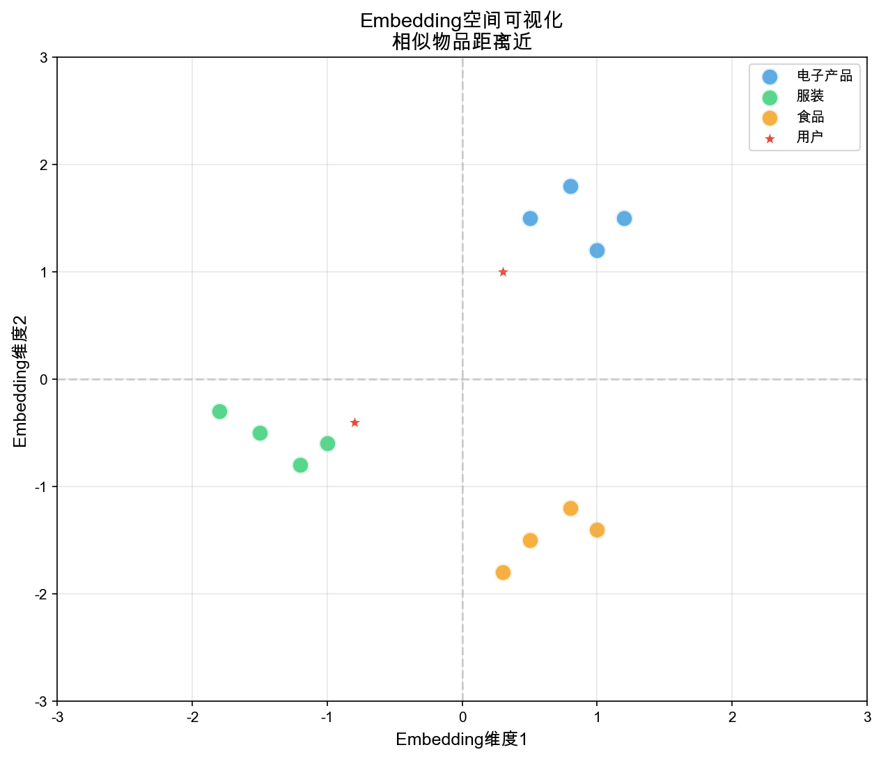
An embedding is a dense, low-dimensional vector representation of a high-dimensional, often sparse, object. In recommendation systems, embeddings transform users and items into continuous vector spaces where similar entities are close together and dissimilar ones are far apart.

Formally, given a set of items \(I = \{i_1, i_2, \dots, i_n\}\), an embedding function\(f: I \rightarrow \mathbb{R}^d\)maps each item\(i\)to a\(d\)-dimensional vector\(\mathbf{e}_i \in \mathbb{R}^d\), where\(d \ll |I|\) (typically\(d \in [64, 512]\)).

Why Embeddings Matter

Dimensionality Reduction: User-item interaction matrices are extremely sparse. For a platform with 100 million users and 10 million items, the interaction matrix has\(10^{15}\)entries, but typically less than 0.01% are observed. Embeddings compress this into manageable dense vectors.

Semantic Relationships: Embeddings capture semantic relationships. If movies\(A\)and\(B\)are similar, their embeddings\(\mathbf{e}_A\)and\(\mathbf{e}_B\)should be close in vector space. This enables: - Similarity search: Find items similar to a given item - Recommendation: Recommend items close to a user's embedding - Clustering: Group similar items together

Computational Efficiency: Dense vectors enable fast similarity computation via dot products or cosine similarity, making real-time recommendation feasible at scale.

The Embedding Learning Objective

The core principle of embedding learning is: items that appear in similar contexts should have similar embeddings. This is formalized through different objectives:

1. Pointwise: Learn embeddings that predict ratings/scores directly
2. Pairwise: Learn embeddings that preserve relative order (item\(A\)preferred over item\(B\))
3. Listwise: Learn embeddings that optimize entire recommendation lists

Most embedding methods optimize a loss function that encourages: - Positive pairs (user-item interactions) to have high similarity - Negative pairs (non-interactions) to have low similarity

Sequence-Based Embeddings: Word2Vec and Item2Vec

Word2Vec: The Foundation

Word2Vec, introduced by Mikolov et al. in 2013, learns word embeddings by predicting words from their context. It comes in two architectures:

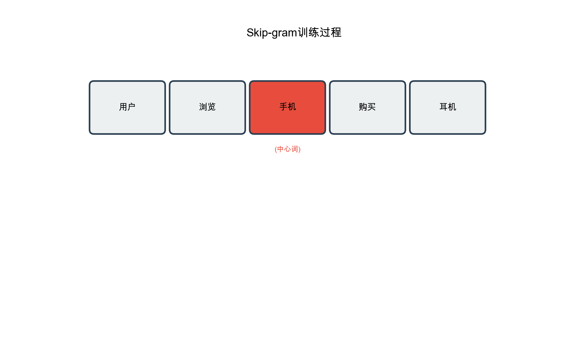
1. Skip-gram: Predict context words from a target word
2. CBOW (Continuous Bag of Words): Predict target word from context words

For recommendation systems, we adapt Word2Vec to learn item embeddings from user interaction sequences.

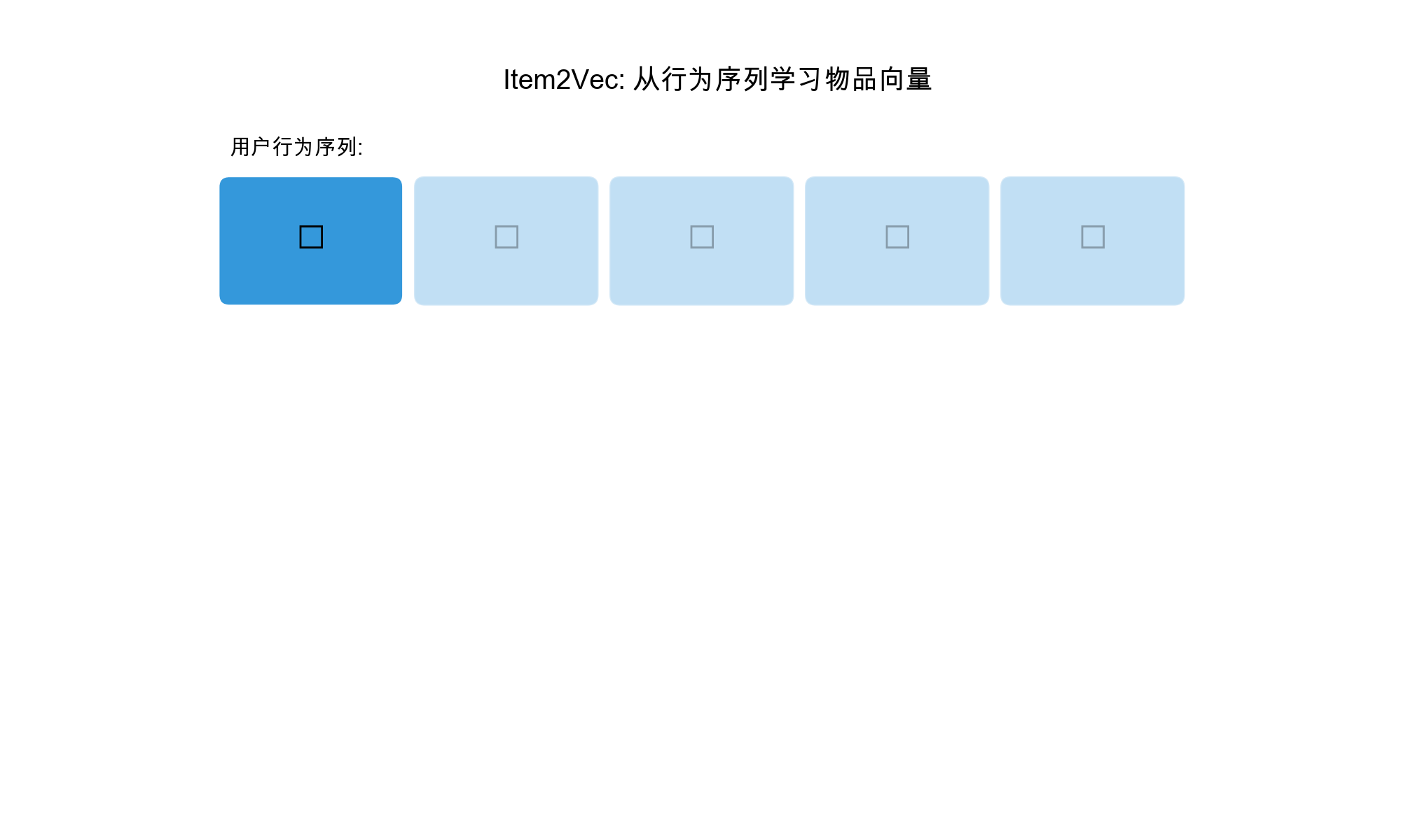
Item2Vec: Adapting Word2Vec for Recommendations

Item2Vec treats user interaction sequences as "sentences" and items as "words." If a user's interaction sequence is\([i_1, i_2, i_3, i_4]\), we learn embeddings such that items appearing close together have similar embeddings.

Key Insight: Items frequently co-occurring in user sequences are likely similar and should be recommended together.

Skip-gram Objective for Item2Vec

Given a sequence of items\(S = [i_1, i_2, \dots, i_T]\), the Skip-gram objective maximizes:\[L = \sum_{t=1}^{T} \sum_{-c \leq j \leq c, j \ne 0} \log p(i_{t+j} | i_t)\]where\(c\)is the context window size, and the probability is defined using softmax:\[p(i_{t+j} | i_t) = \frac{\exp(\mathbf{e}_{i_t}^T \mathbf{e}_{i_{t+j }}')}{\sum_{k=1}^{|I|} \exp(\mathbf{e}_{i_t}^T \mathbf{e}_k')}\]Here,\(\mathbf{e}_i\)is the embedding of item\(i\) (input), and\(\mathbf{e}_i'\)is the context embedding (output). In practice, we often use only one set of embeddings.

Negative Sampling

Computing the full softmax over millions of items is computationally expensive. Negative sampling approximates the objective by sampling negative examples:\[L = \sum_{t=1}^{T} \sum_{-c \leq j \leq c, j \ne 0} \left[ \log \sigma(\mathbf{e}_{i_t}^T \mathbf{e}_{i_{t+j }}') + \sum_{k=1}^{K} \mathbb{E}_{i_k \sim P_n} \log \sigma(-\mathbf{e}_{i_t}^T \mathbf{e}_{i_k}') \right]\]where\(\sigma(x) = 1/(1 + e^{-x})\)is the sigmoid function, and\(P_n\)is the noise distribution (typically unigram distribution raised to\(3/4\)power).

Implementation: Item2Vec with Negative Sampling

Problem Background

In recommendation systems, learning effective item representations is a core challenge. Traditional collaborative filtering methods require explicit user-item interaction matrices, but in practice, we often only have user behavior sequences (e.g., click sequences, purchase sequences). These sequences contain rich co-occurrence information: if two items frequently appear in the same user's behavior sequence, they likely share similar properties or satisfy similar user needs. However, extracting semantic representations from these sequences and capturing item similarities remains challenging.

Solution Approach

Item2Vec adapts Word2Vec's approach to recommendation systems by treating user behavior sequences as "sentences" and items as "words." The core insight is that if two items frequently co-occur in sequences (appear in nearby positions), their embedding vectors should be similar. Specifically, Item2Vec uses the Skip-gram architecture: for each center item in a sequence, the model learns to predict its context items (other items within a window). By maximizing similarity for positive pairs and minimizing similarity for negative pairs, the model learns item vector representations where semantically similar items are closer in vector space.

Design Considerations

When implementing Item2Vec, several key design decisions must be considered:

1. Two Embedding Matrices: Similar to Word2Vec, we use two independent embedding matrices — center item embeddings and context item embeddings. This design provides greater model capacity, allowing more flexible learning of different roles. Ultimately, we only use the center item embeddings as the final item representations.

2. Negative Sampling Strategy: Computing the full softmax over all items is computationally expensive when the number of items is large. Negative sampling approximates the objective by randomly sampling a small number of negative examples (typically 5-20), dramatically improving training efficiency. The negative sampling distribution uses the 3/4 power of item frequencies, avoiding over-sampling of high-frequency items while giving low-frequency items learning opportunities.

3. Window Size Selection: The context window size determines how far co-occurrence relationships are considered. A small window (e.g., 1-2) only captures local co-occurrence, while a large window (e.g., 10+) may introduce noise. Typically, window sizes are set to 3-5, balancing co-occurrence capture and computational efficiency.

4. Numerical Stability: Dot product computations may produce large values, causing sigmoid function overflow. Scores must be clamped to a reasonable range (e.g., [-10, 10]) before computing the loss.

import numpy as np
import torch
import torch.nn as nn
import torch.optim as optim
from collections import Counter
import random

class Item2Vec(nn.Module):
    """
    Item2Vec model using Skip-gram with Negative Sampling.
    """
    def __init__(self, vocab_size, embedding_dim, num_negatives=5):
        super(Item2Vec, self).__init__()
        self.vocab_size = vocab_size
        self.embedding_dim = embedding_dim
        self.num_negatives = num_negatives
        
        # Input and output embeddings (can share weights)
        self.input_embeddings = nn.Embedding(vocab_size, embedding_dim)
        self.output_embeddings = nn.Embedding(vocab_size, embedding_dim)
        
        # Initialize embeddings
        nn.init.xavier_uniform_(self.input_embeddings.weight)
        nn.init.xavier_uniform_(self.output_embeddings.weight)
        
    def forward(self, target, context, negatives):
        """
        Args:
            target: (batch_size,) - target item indices
            context: (batch_size,) - context item indices
            negatives: (batch_size, num_negatives) - negative sample indices
        """
        # Get embeddings
        target_emb = self.input_embeddings(target)  # (batch_size, embedding_dim)
        context_emb = self.output_embeddings(context)  # (batch_size, embedding_dim)
        neg_emb = self.output_embeddings(negatives)  # (batch_size, num_negatives, embedding_dim)
        
        # Positive pairs: target and context
        pos_score = torch.sum(target_emb * context_emb, dim=1)  # (batch_size,)
        pos_loss = -torch.log(torch.sigmoid(pos_score) + 1e-10)
        
        # Negative pairs: target and negative samples
        neg_scores = torch.bmm(
            target_emb.unsqueeze(1),  # (batch_size, 1, embedding_dim)
            neg_emb.transpose(1, 2)   # (batch_size, embedding_dim, num_negatives)
        ).squeeze(1)  # (batch_size, num_negatives)
        neg_loss = -torch.sum(torch.log(torch.sigmoid(-neg_scores) + 1e-10), dim=1)
        
        return pos_loss + neg_loss
    
    def get_item_embedding(self, item_id):
        """Get embedding for an item."""
        return self.input_embeddings(torch.LongTensor([item_id])).detach().numpy()[0]

def build_vocab(sequences):
    """Build vocabulary from sequences."""
    item_counts = Counter()
    for seq in sequences:
        item_counts.update(seq)
    
    # Create item to index mapping
    vocab = {item: idx for idx, item in enumerate(item_counts.keys())}
    return vocab, item_counts

def generate_training_pairs(sequences, vocab, window_size=5):
    """Generate (target, context) pairs from sequences."""
    pairs = []
    for seq in sequences:
        # Convert items to indices
        indices = [vocab[item] for item in seq if item in vocab]
        
        for i, target in enumerate(indices):
            # Context window
            start = max(0, i - window_size)
            end = min(len(indices), i + window_size + 1)
            
            for j in range(start, end):
                if j != i:
                    pairs.append((target, indices[j]))
    
    return pairs

def sample_negatives(item_counts, num_samples, num_negatives=5):
    """Sample negative items based on unigram distribution."""
    # Unigram distribution raised to 3/4 power
    items = list(item_counts.keys())
    probs = np.array([item_counts[item] ** 0.75 for item in items])
    probs = probs / probs.sum()
    
    negatives = np.random.choice(len(items), size=(num_samples, num_negatives), p=probs)
    return negatives

# Example usage
if __name__ == "__main__":
    # Sample user sequences
    sequences = [
        [1, 2, 3, 4, 5],
        [2, 3, 4, 6, 7],
        [1, 3, 5, 8, 9],
        [4, 5, 6, 10, 11],
    ]
    
    # Build vocabulary
    vocab, item_counts = build_vocab(sequences)
    vocab_size = len(vocab)
    
    # Generate training pairs
    pairs = generate_training_pairs(sequences, vocab, window_size=2)
    
    # Initialize model
    model = Item2Vec(vocab_size=vocab_size, embedding_dim=64, num_negatives=5)
    optimizer = optim.Adam(model.parameters(), lr=0.001)
    
    # Training loop
    batch_size = 32
    num_epochs = 10
    
    for epoch in range(num_epochs):
        total_loss = 0
        random.shuffle(pairs)
        
        for i in range(0, len(pairs), batch_size):
            batch_pairs = pairs[i:i+batch_size]
            
            targets = torch.LongTensor([p[0] for p in batch_pairs])
            contexts = torch.LongTensor([p[1] for p in batch_pairs])
            negatives = torch.LongTensor(
                sample_negatives(item_counts, len(batch_pairs), num_negatives=5)
            )
            
            optimizer.zero_grad()
            loss = model(targets, contexts, negatives)
            loss = loss.mean()
            loss.backward()
            optimizer.step()
            
            total_loss += loss.item()
        
        print(f"Epoch {epoch+1}/{num_epochs}, Loss: {total_loss/len(pairs)*batch_size:.4f}")
    
    # Get embeddings
    item_embedding = model.get_item_embedding(0)
    print(f"Embedding for item 0: {item_embedding[:5]}...")

Key Points Interpretation

The Item2Vec implementation includes several key components, each with specific roles:

1. Sequence Construction and Window Sampling: User historical interactions are sorted chronologically to form item sequences, which serve as the foundation data. For each center item in a sequence, we extract other items within its window as context. window_size=2 means considering 2 items before and after, capturing local co-occurrence without introducing excessive noise. Window size selection requires balancing co-occurrence capture and computational efficiency: larger windows generate more training samples but may introduce irrelevant co-occurrences.

2. Negative Sampling Mechanism: Negative sampling is key to Item2Vec's training efficiency. Each positive pair (center item-context item) requires multiple negative pairs (center item-random item). num_negatives=5 means 5 negative samples per positive sample, typically set between 5-20. More negative samples improve the model's ability to distinguish dissimilar items but linearly increase training time.

3. Two Embedding Matrices: Center items and context items use independent embedding matrices, following Word2Vec's design. This design provides greater model capacity, allowing learning of different role representations. Although this increases parameters, experiments show this design improves model performance. Ultimately, we only use center item embeddings as final item representations.

4. Loss Function Design: The negative log-likelihood loss maximizes sigmoid(dot product) for positive samples and minimizes sigmoid(dot product) for negative samples. This design increases dot products for similar items and decreases them for dissimilar items, learning meaningful embeddings.

Design Trade-offs

In Item2Vec's implementation, several design trade-offs exist:

1. Window Size vs Computational Efficiency: Larger windows capture more distant co-occurrence relationships but quadratically increase training samples (O(n ²)). Typically, window sizes are set to 3-5, balancing effectiveness and efficiency.

2. Negative Sample Count vs Training Time: More negative samples improve the model's ability to distinguish negative samples but linearly increase per-batch computation time. Typically set to 5-20, balancing effectiveness and efficiency.

3. Embedding Dimension vs Expressiveness: Higher dimensions provide stronger model expressiveness but increase parameters and may cause overfitting. Typically set to 64-256 dimensions, chosen based on item count and computational resources.

4. Frequency Distribution vs Uniform Distribution: Negative sampling uses the 3/4 power of frequency distribution, avoiding over-sampling of high-frequency items while giving low-frequency items learning opportunities. Uniform distribution would over-sample low-frequency items; direct frequency would over-sample high-frequency items.

Common Issues

1. How to Handle Cold-Start Items? For new items not in the training set, Item2Vec cannot directly learn their embeddings. Common solutions include: (1) Using item content features (e.g., category, tags) to generate initial embeddings through additional neural networks; (2) Using similar items' embeddings as initialization; (3) Assigning randomly initialized embeddings to new items during training, learning quickly through few interactions.

2. Numerical Overflow Issues: Dot product computations may produce large values (especially when embeddings are not normalized), causing sigmoid function overflow. Code uses torch.clamp to limit scores to [-10, 10], an important numerical stability technique.

3. Negative Sample Duplication: Random negative sampling may sample positive samples (items within the context window). Strictly speaking, positive samples should be excluded, but when item counts are large (e.g., millions), the probability of sampling positive samples is very small (<0.1%) and can be ignored. If item counts are small, positive samples can be excluded during sampling.

4. Inconsistent Sequence Lengths: In practice, user sequence lengths vary greatly, from a few items to hundreds of items. Common approaches include: (1) Truncation: Keep only the most recent N items (e.g., last 50); (2) Padding: Pad short sequences to fixed length; (3) Dynamic batching: Group sequences of similar lengths in the same batch.

5. How to Handle Temporal Information? Item2Vec ignores temporal information in sequences, treating all items within a window equally. If temporal decay is needed, different weights can be assigned to context items at different positions in the loss function, with weights decreasing as distance from the center item increases.

Usage Example

The following example demonstrates how to use Item2Vec for training and obtaining item embeddings:

# Prepare user behavior sequence data
sequences = [
    [0, 1, 2, 3, 4],    # User 1's interaction sequence
    [1, 2, 5, 6, 7],    # User 2's interaction sequence
    [0, 3, 4, 8, 9],    # User 3's interaction sequence
]

# Create trainer and train model
trainer = Item2VecTrainer(
    sequences=sequences,
    vocab_size=12,
    embedding_dim=64,
    window_size=2,
    num_negatives=5,
    batch_size=32,
    learning_rate=0.01
)

# Train model (typically 5-20 epochs)
embeddings = trainer.train(num_epochs=10)

# Use embeddings for similar item recommendation
item_emb = embeddings[0]  # Get item 0's embedding
similarities = [cosine_similarity(item_emb, embeddings[i]) for i in range(12)]
top_k_items = np.argsort(similarities)[::-1][:5]  # Find 5 most similar items

In practice, Item2Vec is typically used as a feature extractor, with learned embeddings used for: (1) Similar item recommendation; (2) Input features for downstream models; (3) Item clustering and visualization analysis.

CBOW Variant for Item2Vec

The CBOW (Continuous Bag of Words) variant predicts the target item from its context:

class Item2VecCBOW(nn.Module):
    """
    Item2Vec CBOW model: predict target from context.
    """
    def __init__(self, vocab_size, embedding_dim, num_negatives=5):
        super(Item2VecCBOW, self).__init__()
        self.vocab_size = vocab_size
        self.embedding_dim = embedding_dim
        self.num_negatives = num_negatives
        
        self.input_embeddings = nn.Embedding(vocab_size, embedding_dim)
        self.output_embeddings = nn.Embedding(vocab_size, embedding_dim)
        
        nn.init.xavier_uniform_(self.input_embeddings.weight)
        nn.init.xavier_uniform_(self.output_embeddings.weight)
    
    def forward(self, context_items, target, negatives):
        """
        Args:
            context_items: (batch_size, context_size) - context item indices
            target: (batch_size,) - target item indices
            negatives: (batch_size, num_negatives) - negative sample indices
        """
        # Average context embeddings
        context_emb = self.input_embeddings(context_items)  # (batch_size, context_size, embedding_dim)
        context_emb = context_emb.mean(dim=1)  # (batch_size, embedding_dim)
        
        # Target embedding
        target_emb = self.output_embeddings(target)  # (batch_size, embedding_dim)
        
        # Negative embeddings
        neg_emb = self.output_embeddings(negatives)  # (batch_size, num_negatives, embedding_dim)
        
        # Positive score
        pos_score = torch.sum(context_emb * target_emb, dim=1)
        pos_loss = -torch.log(torch.sigmoid(pos_score) + 1e-10)
        
        # Negative scores
        neg_scores = torch.bmm(
            context_emb.unsqueeze(1),
            neg_emb.transpose(1, 2)
        ).squeeze(1)
        neg_loss = -torch.sum(torch.log(torch.sigmoid(-neg_scores) + 1e-10), dim=1)
        
        return pos_loss + neg_loss

Graph-Based Embeddings: Node2Vec

Why Graph-Based Embeddings?

While Item2Vec captures sequential patterns, many recommendation scenarios involve complex item relationships that aren't purely sequential. Graph-based embeddings model items as nodes in a graph, where edges represent relationships (co-purchase, co-view, similarity, etc.).

Node2Vec, introduced by Grover and Leskovec in 2016, learns node embeddings by exploring the graph through biased random walks, balancing between breadth-first search (BFS) and depth-first search (DFS) exploration.

Node2Vec Algorithm

Node2Vec uses biased random walks with two parameters: - \(p\)(return parameter): Controls likelihood of returning to previous node - \(q\)(in-out parameter): Controls exploration of distant vs. nearby nodes

The transition probability from node\(v\)to node\(x\)is:\[\alpha_{pq}(t, x) = \begin{cases} \frac{1}{p} & \text{if } d_{tx} = 0 \\ 1 & \text{if } d_{tx} = 1 \\ \frac{1}{q} & \text{if } d_{tx} = 2 \end{cases}\]where\(d_{tx}\)is the shortest path distance between nodes\(t\)(previous node) and\(x\).

• \(p < 1\): More likely to return (BFS-like, local exploration)
• \(p > 1\): Less likely to return (DFS-like, global exploration)
• \(q < 1\): Prefer distant nodes (DFS-like)
• \(q > 1\): Prefer nearby nodes (BFS-like)

Implementation: Node2Vec for Recommendation

Problem Background

In recommendation systems, user-item interactions can be naturally modeled as graph structures: users and items are two types of nodes, and interactions are edges. This graph structure contains rich semantic information: users with similar connections (e.g., purchasing the same items) may have similar interests; items with similar structures (e.g., purchased by similar users) may have similar properties. However, learning effective representations of nodes (users and items) from graph structures, such that similar nodes are closer in vector space, remains challenging. Traditional graph embedding methods (e.g., DeepWalk) use standard random walks to generate node sequences, but this approach cannot flexibly control walk strategies, making it difficult to simultaneously capture local structures (e.g., communities) and global structures (e.g., node roles).

Solution Approach

Node2Vec addresses this by introducing biased random walks. The core idea is to control walk strategies through two parameters p and q, allowing walks to flexibly switch between depth-first search (DFS) and breadth-first search (BFS). Specifically, p (return parameter) controls the probability of returning to the previous node, and q (in-out parameter) controls the probability of exploring nodes far from the starting node. When p is small and q is large, walks tend toward BFS, capturing local community structures; when p is large and q is small, walks tend toward DFS, capturing global structures. Through this flexible walk strategy, Node2Vec generates diverse node sequences, then uses Skip-gram to learn node embeddings, making structurally similar or similarly connected nodes closer in vector space.

Design Considerations

When implementing Node2Vec, several key design decisions must be considered:

1. Biased Walk Strategy: Walk probability calculations must consider the relationships between the previous node, current node, and candidate nodes. For each candidate node, the shortest distance to the previous node must be computed, then different weights assigned based on distance. This design allows walks to flexibly balance local exploration and global exploration.

2. Graph Preprocessing: To accelerate walk generation, neighbor information for each node must be precomputed and stored. This avoids repeated graph structure queries during training, significantly improving walk generation speed. For large-scale graphs, this preprocessing is necessary.

3. Walk Sequence Generation: Multiple walks are performed for each node (typically 10-50), each generating a fixed-length sequence (typically 50-100). More walks capture richer graph structure information but increase computational cost.

4. Skip-gram Training: Generated walk sequences are treated as "sentences," using Skip-gram to learn node embeddings. This is similar to Item2Vec's training process but with different data sources: Item2Vec uses user behavior sequences, while Node2Vec uses graph walk sequences.

import numpy as np
import networkx as nx
from collections import defaultdict
import random

class Node2Vec:
    """
    Node2Vec implementation for learning node embeddings.
    """
    def __init__(self, graph, dimensions=64, walk_length=80, num_walks=10, 
                 p=1.0, q=1.0, window_size=10, num_negatives=5):
        """
        Args:
            graph: NetworkX graph or edge list
            dimensions: Embedding dimension
            walk_length: Length of each random walk
            num_walks: Number of walks per node
            p: Return parameter
            q: In-out parameter
            window_size: Context window size
            num_negatives: Number of negative samples
        """
        self.graph = self._build_graph(graph)
        self.dimensions = dimensions
        self.walk_length = walk_length
        self.num_walks = num_walks
        self.p = p
        self.q = q
        self.window_size = window_size
        self.num_negatives = num_negatives
        
        # Precompute transition probabilities
        self.alias_nodes = {}
        self.alias_edges = {}
        self._precompute_transition_probs()
    
    def _build_graph(self, graph):
        """Build NetworkX graph from input."""
        if isinstance(graph, nx.Graph):
            return graph
        else:
            # Assume edge list: [(u, v, weight), ...]
            G = nx.Graph()
            for edge in graph:
                if len(edge) == 2:
                    G.add_edge(edge[0], edge[1])
                else:
                    G.add_edge(edge[0], edge[1], weight=edge[2])
            return G
    
    def _precompute_transition_probs(self):
        """Precompute transition probabilities for efficient random walks."""
        G = self.graph
        
        # Alias nodes: for unweighted graphs, uniform distribution
        for node in G.nodes():
            unnormalized_probs = [G[node][nbr].get('weight', 1.0) 
                                 for nbr in G.neighbors(node)]
            norm_const = sum(unnormalized_probs)
            normalized_probs = [float(u_prob) / norm_const 
                               for u_prob in unnormalized_probs]
            self.alias_nodes[node] = self._alias_setup(normalized_probs)
        
        # Alias edges: biased transition probabilities
        for edge in G.edges():
            self.alias_edges[(edge[0], edge[1])] = self._get_edge_alias(edge[0], edge[1])
            self.alias_edges[(edge[1], edge[0])] = self._get_edge_alias(edge[1], edge[0])
    
    def _get_edge_alias(self, src, dst):
        """Get alias table for edge (src, dst) considering previous node."""
        G = self.graph
        unnormalized_probs = []
        
        for nbr in G.neighbors(dst):
            if nbr == src:
                # Return to previous node
                unnormalized_probs.append(G[dst][nbr].get('weight', 1.0) / self.p)
            elif G.has_edge(src, nbr):
                # Distance 1 from previous node
                unnormalized_probs.append(G[dst][nbr].get('weight', 1.0))
            else:
                # Distance 2 from previous node
                unnormalized_probs.append(G[dst][nbr].get('weight', 1.0) / self.q)
        
        norm_const = sum(unnormalized_probs)
        normalized_probs = [float(u_prob) / norm_const for u_prob in unnormalized_probs]
        neighbors = list(G.neighbors(dst))
        
        return self._alias_setup(normalized_probs), neighbors
    
    def _alias_setup(self, probs):
        """Set up alias table for efficient sampling."""
        K = len(probs)
        q = np.zeros(K)
        J = np.zeros(K, dtype=np.int32)
        
        smaller = []
        larger = []
        
        for kk, prob in enumerate(probs):
            q[kk] = K * prob
            if q[kk] < 1.0:
                smaller.append(kk)
            else:
                larger.append(kk)
        
        while len(smaller) > 0 and len(larger) > 0:
            small = smaller.pop()
            large = larger.pop()
            
            J[small] = large
            q[large] = q[large] + q[small] - 1.0
            
            if q[large] < 1.0:
                smaller.append(large)
            else:
                larger.append(large)
        
        return J, q
    
    def _alias_draw(self, J, q):
        """Draw sample from alias table."""
        K = len(J)
        kk = int(np.floor(np.random.rand() * K))
        if np.random.rand() < q[kk]:
            return kk
        else:
            return J[kk]
    
    def node2vec_walk(self, start_node):
        """Generate a single biased random walk."""
        G = self.graph
        walk = [start_node]
        
        while len(walk) < self.walk_length:
            cur = walk[-1]
            cur_nbrs = list(G.neighbors(cur))
            
            if len(cur_nbrs) > 0:
                if len(walk) == 1:
                    # First step: uniform sampling
                    alias, neighbors = self.alias_nodes[cur]
                    walk.append(neighbors[self._alias_draw(alias, self.alias_nodes[cur][1])])
                else:
                    # Use edge alias with previous node
                    prev = walk[-2]
                    alias, neighbors = self.alias_edges[(prev, cur)]
                    next_idx = self._alias_draw(alias, self.alias_edges[(prev, cur)][1])
                    walk.append(neighbors[next_idx])
            else:
                break
        
        return walk
    
    def simulate_walks(self):
        """Generate random walks for all nodes."""
        walks = []
        nodes = list(self.graph.nodes())
        
        for _ in range(self.num_walks):
            random.shuffle(nodes)
            for node in nodes:
                walks.append(self.node2vec_walk(node))
        
        return walks
    
    def learn_embeddings(self, walks):
        """Learn embeddings from walks using Word2Vec-style training."""
        # Convert walks to sequences and train Item2Vec
        # This is a simplified version; in practice, use gensim Word2Vec
        from gensim.models import Word2Vec
        
        # Convert node IDs to strings for gensim
        walks_str = [[str(node) for node in walk] for walk in walks]
        
        model = Word2Vec(
            walks_str,
            vector_size=self.dimensions,
            window=self.window_size,
            min_count=0,
            sg=1,  # Skip-gram
            negative=self.num_negatives,
            workers=4
        )
        
        # Extract embeddings
        embeddings = {}
        for node in self.graph.nodes():
            embeddings[node] = model.wv[str(node)]
        
        return embeddings

# Example usage
if __name__ == "__main__":
    # Create a sample graph (e.g., co-purchase graph)
    G = nx.Graph()
    G.add_edges_from([
        (0, 1), (0, 2), (1, 2), (1, 3),
        (2, 4), (3, 4), (3, 5), (4, 5)
    ])
    
    # Initialize Node2Vec
    node2vec = Node2Vec(
        graph=G,
        dimensions=64,
        walk_length=10,
        num_walks=5,
        p=1.0,
        q=1.0
    )
    
    # Generate walks
    walks = node2vec.simulate_walks()
    print(f"Generated {len(walks)} walks")
    print(f"Sample walk: {walks[0]}")
    
    # Learn embeddings
    embeddings = node2vec.learn_embeddings(walks)
    print(f"Learned embeddings for {len(embeddings)} nodes")
    print(f"Embedding for node 0: {embeddings[0][:5]}...")

Building Item Graphs for Recommendation

To apply Node2Vec to recommendations, we need to construct item graphs:

def build_item_graph_from_interactions(interactions, similarity_threshold=0.5):
    """
    Build item graph from user-item interactions.
    
    Args:
        interactions: List of (user_id, item_id) tuples
        similarity_threshold: Minimum similarity to create edge
    """
    from collections import defaultdict
    
    # Build user-item matrix
    user_items = defaultdict(set)
    item_users = defaultdict(set)
    
    for user_id, item_id in interactions:
        user_items[user_id].add(item_id)
        item_users[item_id].add(user_id)
    
    # Compute item-item similarity (Jaccard)
    G = nx.Graph()
    items = list(item_users.keys())
    
    for i, item1 in enumerate(items):
        G.add_node(item1)
        for item2 in items[i+1:]:
            users1 = item_users[item1]
            users2 = item_users[item2]
            
            # Jaccard similarity
            intersection = len(users1 & users2)
            union = len(users1 | users2)
            
            if union > 0:
                similarity = intersection / union
                if similarity >= similarity_threshold:
                    G.add_edge(item1, item2, weight=similarity)
    
    return G

# Example: Build graph from interactions
interactions = [
    (0, 1), (0, 2), (0, 3),
    (1, 2), (1, 3), (1, 4),
    (2, 3), (2, 4), (2, 5),
    (3, 4), (3, 5),
]

item_graph = build_item_graph_from_interactions(interactions, similarity_threshold=0.3)
print(f"Graph has {item_graph.number_of_nodes()} nodes and {item_graph.number_of_edges()} edges")

Two-Tower Models: Separate User and Item Embeddings

Architecture Overview

Two-tower models learn separate embedding towers for users and items, then compute similarity via dot product or cosine similarity. This architecture is scalable and enables efficient serving.

Key Components: 1. User Tower: Encodes user features (ID, demographics, behavior history) into user embedding 2. Item Tower: Encodes item features (ID, content, metadata) into item embedding 3. Similarity Function: Computes similarity between user and item embeddings

Advantages of Two-Tower Architecture

• Scalability: Pre-compute item embeddings offline, compute user embeddings online
• Efficiency: Fast similarity search via approximate nearest neighbor (ANN) algorithms
• Flexibility: Can incorporate rich features in both towers
• Cold Start: Can handle new users/items through feature-based towers

Deep Structured Semantic Models (DSSM)

DSSM Architecture

DSSM (Deep Structured Semantic Model), introduced by Microsoft in 2013, was originally designed for web search but has been widely adopted for recommendation systems.

Architecture: 1. Query Tower: Multi-layer neural network encoding query (user) features 2. Document Tower: Multi-layer neural network encoding document (item) features 3. Similarity: Cosine similarity between query and document embeddings 4. Training: Maximize similarity for positive pairs, minimize for negative pairs

Mathematical Formulation

Given a user\(u\)with features\(\mathbf{x}_u\)and an item\(i\)with features\(\mathbf{x}_i\):\[\mathbf{e}_u = f_u(\mathbf{x}_u; \theta_u)$ \]\(\mathbf{e}_i = f_i(\mathbf{x}_i; \theta_i)\) $

\[s(u, i) = \cos(\mathbf{e}_u, \mathbf{e}_i) = \frac{\mathbf{e}_u^T \mathbf{e}_i}{|\mathbf{e}_u| \cdot |\mathbf{e}_i|}\]The training objective maximizes the probability of positive pairs:\[P(i | u) = \frac{\exp(s(u, i))}{\sum_{j \in \mathcal{N}_u} \exp(s(u, j))}\]where\(\mathcal{N}_u\)includes positive items and sampled negatives.

Implementation: DSSM for Recommendation

import torch
import torch.nn as nn
import torch.nn.functional as F

class DSSM(nn.Module):
    """
    Deep Structured Semantic Model for recommendation.
    """
    def __init__(self, user_feature_dim, item_feature_dim, embedding_dim=128,
                 hidden_dims=[256, 128]):
        """
        Args:
            user_feature_dim: Dimension of user feature vector
            item_feature_dim: Dimension of item feature vector
            embedding_dim: Output embedding dimension
            hidden_dims: List of hidden layer dimensions
        """
        super(DSSM, self).__init__()
        
        # User tower
        user_layers = []
        input_dim = user_feature_dim
        for hidden_dim in hidden_dims:
            user_layers.append(nn.Linear(input_dim, hidden_dim))
            user_layers.append(nn.ReLU())
            user_layers.append(nn.BatchNorm1d(hidden_dim))
            input_dim = hidden_dim
        user_layers.append(nn.Linear(input_dim, embedding_dim))
        self.user_tower = nn.Sequential(*user_layers)
        
        # Item tower
        item_layers = []
        input_dim = item_feature_dim
        for hidden_dim in hidden_dims:
            item_layers.append(nn.Linear(input_dim, hidden_dim))
            item_layers.append(nn.ReLU())
            item_layers.append(nn.BatchNorm1d(hidden_dim))
            input_dim = hidden_dim
        item_layers.append(nn.Linear(input_dim, embedding_dim))
        self.item_tower = nn.Sequential(*item_layers)
    
    def forward(self, user_features, item_features):
        """
        Args:
            user_features: (batch_size, user_feature_dim)
            item_features: (batch_size, item_feature_dim)
        Returns:
            user_emb: (batch_size, embedding_dim)
            item_emb: (batch_size, embedding_dim)
            similarity: (batch_size,)
        """
        user_emb = self.user_tower(user_features)
        item_emb = self.item_tower(item_features)
        
        # L2 normalize for cosine similarity
        user_emb = F.normalize(user_emb, p=2, dim=1)
        item_emb = F.normalize(item_emb, p=2, dim=1)
        
        # Cosine similarity
        similarity = (user_emb * item_emb).sum(dim=1)
        
        return user_emb, item_emb, similarity
    
    def get_user_embedding(self, user_features):
        """Get user embedding."""
        user_emb = self.user_tower(user_features)
        return F.normalize(user_emb, p=2, dim=1)
    
    def get_item_embedding(self, item_features):
        """Get item embedding."""
        item_emb = self.item_tower(item_features)
        return F.normalize(item_emb, p=2, dim=1)

class DSSMLoss(nn.Module):
    """
    Loss function for DSSM training with negative sampling.
    """
    def __init__(self, temperature=1.0):
        """
        Args:
            temperature: Temperature parameter for softmax
        """
        super(DSSMLoss, self).__init__()
        self.temperature = temperature
    
    def forward(self, user_emb, pos_item_emb, neg_item_emb):
        """
        Args:
            user_emb: (batch_size, embedding_dim)
            pos_item_emb: (batch_size, embedding_dim)
            neg_item_emb: (batch_size, num_negatives, embedding_dim)
        """
        # Positive similarity
        pos_sim = (user_emb * pos_item_emb).sum(dim=1) / self.temperature  # (batch_size,)
        
        # Negative similarities
        neg_sim = torch.bmm(
            user_emb.unsqueeze(1),  # (batch_size, 1, embedding_dim)
            neg_item_emb.transpose(1, 2)  # (batch_size, embedding_dim, num_negatives)
        ).squeeze(1) / self.temperature  # (batch_size, num_negatives)
        
        # Log-softmax loss
        logits = torch.cat([pos_sim.unsqueeze(1), neg_sim], dim=1)  # (batch_size, 1 + num_negatives)
        loss = -F.log_softmax(logits, dim=1)[:, 0].mean()
        
        return loss

# Example usage
if __name__ == "__main__":
    batch_size = 32
    user_feature_dim = 100
    item_feature_dim = 50
    embedding_dim = 128
    num_negatives = 5
    
    # Initialize model
    model = DSSM(
        user_feature_dim=user_feature_dim,
        item_feature_dim=item_feature_dim,
        embedding_dim=embedding_dim,
        hidden_dims=[256, 128]
    )
    
    # Sample data
    user_features = torch.randn(batch_size, user_feature_dim)
    pos_item_features = torch.randn(batch_size, item_feature_dim)
    neg_item_features = torch.randn(batch_size, num_negatives, item_feature_dim)
    
    # Forward pass
    user_emb, pos_item_emb, similarity = model(user_features, pos_item_features)
    
    # Get negative item embeddings
    neg_item_emb = model.get_item_embedding(
        neg_item_features.view(-1, item_feature_dim)
    ).view(batch_size, num_negatives, embedding_dim)
    
    # Compute loss
    criterion = DSSMLoss(temperature=1.0)
    loss = criterion(user_emb, pos_item_emb, neg_item_emb)
    
    print(f"User embedding shape: {user_emb.shape}")
    print(f"Item embedding shape: {pos_item_emb.shape}")
    print(f"Similarity shape: {similarity.shape}")
    print(f"Loss: {loss.item():.4f}")

Feature Engineering for DSSM

DSSM can incorporate various features:

class FeatureEncoder:
    """
    Encode various features for DSSM input.
    """
    def __init__(self, vocab_sizes=None):
        """
        Args:
            vocab_sizes: Dict mapping feature names to vocabulary sizes
        """
        self.vocab_sizes = vocab_sizes or {}
        self.embeddings = {}
        
        # Initialize embeddings for categorical features
        for feat_name, vocab_size in self.vocab_sizes.items():
            self.embeddings[feat_name] = nn.Embedding(vocab_size, 16)
    
    def encode_user_features(self, user_data):
        """
        Encode user features into dense vector.
        
        Args:
            user_data: Dict with keys like 'user_id', 'age', 'gender', 'history'
        """
        features = []
        
        # User ID embedding
        if 'user_id' in user_data:
            user_id_emb = self.embeddings['user_id'](user_data['user_id'])
            features.append(user_id_emb)
        
        # Numerical features (normalized)
        if 'age' in user_data:
            age_normalized = user_data['age'] / 100.0  # Normalize
            features.append(age_normalized.unsqueeze(1))
        
        # Categorical features
        if 'gender' in user_data:
            gender_emb = self.embeddings['gender'](user_data['gender'])
            features.append(gender_emb)
        
        # Historical behavior (average of item embeddings)
        if 'history' in user_data:
            # Assume history is a list of item IDs
            history_emb = self.embeddings['item_id'](user_data['history'])
            history_emb = history_emb.mean(dim=1)  # Average pooling
            features.append(history_emb)
        
        return torch.cat(features, dim=1)
    
    def encode_item_features(self, item_data):
        """
        Encode item features into dense vector.
        
        Args:
            item_data: Dict with keys like 'item_id', 'category', 'price'
        """
        features = []
        
        # Item ID embedding
        if 'item_id' in item_data:
            item_id_emb = self.embeddings['item_id'](item_data['item_id'])
            features.append(item_id_emb)
        
        # Category embedding
        if 'category' in item_data:
            category_emb = self.embeddings['category'](item_data['category'])
            features.append(category_emb)
        
        # Numerical features
        if 'price' in item_data:
            price_normalized = torch.log(item_data['price'] + 1) / 10.0
            features.append(price_normalized.unsqueeze(1))
        
        return torch.cat(features, dim=1)

YouTube DNN: Deep Neural Network for Recommendations

YouTube DNN Architecture

YouTube DNN, introduced in 2016, is a two-tower model specifically designed for large-scale video recommendation. It addresses several key challenges:

1. Extreme Scale: Millions of videos, billions of users
2. Freshness: New videos uploaded constantly
3. Implicit Feedback: Watch time, clicks, not explicit ratings
4. Real-time Serving: Low-latency requirements

Architecture Details

User Tower: - Input: User watch history (sequence of video IDs) - Processing: Average pooling over watched video embeddings - Additional features: User demographics, search queries - Output: User embedding

Item Tower: - Input: Video features (ID, category, tags, etc.) - Processing: Concatenate and pass through MLP - Output: Item embedding

Training: - Objective: Predict next video to watch - Loss: Weighted logistic regression (weighted by watch time) - Negative sampling: Sample from entire video corpus

Implementation: YouTube DNN

import torch
import torch.nn as nn
import torch.nn.functional as F

class YouTubeDNN(nn.Module):
    """
    YouTube DNN model for video recommendation.
    """
    def __init__(self, num_videos, num_categories, embedding_dim=64,
                 user_hidden_dims=[256, 128], item_hidden_dims=[128, 64]):
        """
        Args:
            num_videos: Number of videos (for video ID embedding)
            num_categories: Number of video categories
            embedding_dim: Output embedding dimension
            user_hidden_dims: Hidden dimensions for user tower
            item_hidden_dims: Hidden dimensions for item tower
        """
        super(YouTubeDNN, self).__init__()
        
        self.embedding_dim = embedding_dim
        
        # Video embedding (shared between user and item towers)
        self.video_embedding = nn.Embedding(num_videos, embedding_dim)
        self.category_embedding = nn.Embedding(num_categories, 16)
        
        # User tower
        user_input_dim = embedding_dim + 16  # Video embedding + category embedding
        user_layers = []
        for hidden_dim in user_hidden_dims:
            user_layers.append(nn.Linear(user_input_dim, hidden_dim))
            user_layers.append(nn.ReLU())
            user_input_dim = hidden_dim
        user_layers.append(nn.Linear(user_input_dim, embedding_dim))
        self.user_tower = nn.Sequential(*user_layers)
        
        # Item tower
        item_input_dim = embedding_dim + 16  # Video embedding + category embedding
        item_layers = []
        for hidden_dim in item_hidden_dims:
            item_layers.append(nn.Linear(item_input_dim, hidden_dim))
            item_layers.append(nn.ReLU())
            item_input_dim = hidden_dim
        item_layers.append(nn.Linear(item_input_dim, embedding_dim))
        self.item_tower = nn.Sequential(*item_layers)
    
    def forward(self, user_history, user_history_categories, 
                item_id, item_category):
        """
        Args:
            user_history: (batch_size, history_length) - video IDs in history
            user_history_categories: (batch_size, history_length) - categories
            item_id: (batch_size,) - target video ID
            item_category: (batch_size,) - target video category
        Returns:
            user_emb: (batch_size, embedding_dim)
            item_emb: (batch_size, embedding_dim)
            logits: (batch_size,)
        """
        batch_size = user_history.size(0)
        
        # User tower: average pooling over history
        history_emb = self.video_embedding(user_history)  # (batch_size, history_length, embedding_dim)
        history_cat_emb = self.category_embedding(user_history_categories)  # (batch_size, history_length, 16)
        
        # Average pooling
        history_emb = history_emb.mean(dim=1)  # (batch_size, embedding_dim)
        history_cat_emb = history_cat_emb.mean(dim=1)  # (batch_size, 16)
        
        user_features = torch.cat([history_emb, history_cat_emb], dim=1)
        user_emb = self.user_tower(user_features)
        user_emb = F.normalize(user_emb, p=2, dim=1)
        
        # Item tower
        item_emb_base = self.video_embedding(item_id)  # (batch_size, embedding_dim)
        item_cat_emb = self.category_embedding(item_category)  # (batch_size, 16)
        
        item_features = torch.cat([item_emb_base, item_cat_emb], dim=1)
        item_emb = self.item_tower(item_features)
        item_emb = F.normalize(item_emb, p=2, dim=1)
        
        # Similarity
        logits = (user_emb * item_emb).sum(dim=1)
        
        return user_emb, item_emb, logits
    
    def get_user_embedding(self, user_history, user_history_categories):
        """Get user embedding for serving."""
        history_emb = self.video_embedding(user_history)
        history_cat_emb = self.category_embedding(user_history_categories)
        
        history_emb = history_emb.mean(dim=1)
        history_cat_emb = history_cat_emb.mean(dim=1)
        
        user_features = torch.cat([history_emb, history_cat_emb], dim=1)
        user_emb = self.user_tower(user_features)
        return F.normalize(user_emb, p=2, dim=1)
    
    def get_item_embedding(self, item_id, item_category):
        """Get item embedding for serving."""
        item_emb_base = self.video_embedding(item_id)
        item_cat_emb = self.category_embedding(item_category)
        
        item_features = torch.cat([item_emb_base, item_cat_emb], dim=1)
        item_emb = self.item_tower(item_features)
        return F.normalize(item_emb, p=2, dim=1)

class YouTubeDNNLoss(nn.Module):
    """
    Weighted logistic loss for YouTube DNN.
    """
    def __init__(self):
        super(YouTubeDNNLoss, self).__init__()
    
    def forward(self, logits, labels, weights=None):
        """
        Args:
            logits: (batch_size,) - prediction logits
            labels: (batch_size,) - binary labels (1 for positive, 0 for negative)
            weights: (batch_size,) - sample weights (e.g., watch time)
        """
        if weights is None:
            weights = torch.ones_like(labels)
        
        # Weighted binary cross-entropy
        loss = F.binary_cross_entropy_with_logits(
            logits, labels.float(), weight=weights, reduction='none'
        )
        
        return loss.mean()

# Example usage
if __name__ == "__main__":
    batch_size = 32
    history_length = 50
    num_videos = 10000
    num_categories = 100
    embedding_dim = 64
    
    model = YouTubeDNN(
        num_videos=num_videos,
        num_categories=num_categories,
        embedding_dim=embedding_dim
    )
    
    # Sample data
    user_history = torch.randint(0, num_videos, (batch_size, history_length))
    user_history_categories = torch.randint(0, num_categories, (batch_size, history_length))
    item_id = torch.randint(0, num_videos, (batch_size,))
    item_category = torch.randint(0, num_categories, (batch_size,))
    labels = torch.randint(0, 2, (batch_size,)).float()
    weights = torch.rand(batch_size)  # Watch time weights
    
    # Forward pass
    user_emb, item_emb, logits = model(
        user_history, user_history_categories, item_id, item_category
    )
    
    # Compute loss
    criterion = YouTubeDNNLoss()
    loss = criterion(logits, labels, weights)
    
    print(f"User embedding shape: {user_emb.shape}")
    print(f"Item embedding shape: {item_emb.shape}")
    print(f"Logits shape: {logits.shape}")
    print(f"Loss: {loss.item():.4f}")

Handling Variable-Length Sequences

YouTube DNN uses average pooling, but we can also use attention or RNNs:

class YouTubeDNNWithAttention(nn.Module):
    """
    YouTube DNN with attention mechanism for history.
    """
    def __init__(self, num_videos, num_categories, embedding_dim=64):
        super(YouTubeDNNWithAttention, self).__init__()
        
        self.video_embedding = nn.Embedding(num_videos, embedding_dim)
        self.category_embedding = nn.Embedding(num_categories, 16)
        
        # Attention mechanism
        self.attention = nn.MultiheadAttention(
            embed_dim=embedding_dim,
            num_heads=4,
            batch_first=True
        )
        
        # User tower
        self.user_tower = nn.Sequential(
            nn.Linear(embedding_dim + 16, 256),
            nn.ReLU(),
            nn.Linear(256, embedding_dim)
        )
        
        # Item tower (same as before)
        self.item_tower = nn.Sequential(
            nn.Linear(embedding_dim + 16, 128),
            nn.ReLU(),
            nn.Linear(128, embedding_dim)
        )
    
    def forward(self, user_history, user_history_categories,
                item_id, item_category):
        # User tower with attention
        history_emb = self.video_embedding(user_history)  # (batch_size, seq_len, embedding_dim)
        
        # Self-attention over history
        attended_emb, _ = self.attention(history_emb, history_emb, history_emb)
        history_emb = attended_emb.mean(dim=1)  # (batch_size, embedding_dim)
        
        history_cat_emb = self.category_embedding(user_history_categories).mean(dim=1)
        
        user_features = torch.cat([history_emb, history_cat_emb], dim=1)
        user_emb = self.user_tower(user_features)
        user_emb = F.normalize(user_emb, p=2, dim=1)
        
        # Item tower (same as before)
        item_emb_base = self.video_embedding(item_id)
        item_cat_emb = self.category_embedding(item_category)
        item_features = torch.cat([item_emb_base, item_cat_emb], dim=1)
        item_emb = self.item_tower(item_features)
        item_emb = F.normalize(item_emb, p=2, dim=1)
        
        logits = (user_emb * item_emb).sum(dim=1)
        
        return user_emb, item_emb, logits

Negative Sampling Strategies

Why Negative Sampling?

In recommendation systems, we have far more negative examples (non-interactions) than positive ones. Computing loss over all negatives is computationally expensive. Negative sampling selects a small subset of negatives for training.

Common Negative Sampling Strategies

1. Uniform Random Sampling

Sample negatives uniformly from all items:

def uniform_negative_sampling(item_set, num_negatives, exclude_items=None):
    """
    Uniform random negative sampling.
    
    Args:
        item_set: Set of all item IDs
        num_negatives: Number of negatives to sample
        exclude_items: Set of items to exclude (e.g., positive items)
    """
    if exclude_items:
        candidates = list(item_set - exclude_items)
    else:
        candidates = list(item_set)
    
    negatives = random.sample(candidates, min(num_negatives, len(candidates)))
    return negatives

2. Popularity-Based Sampling

Sample negatives proportional to item popularity (unigram distribution):

def popularity_negative_sampling(item_popularity, num_negatives, exclude_items=None):
    """
    Sample negatives based on item popularity.
    
    Args:
        item_popularity: Dict mapping item_id to popularity count
        num_negatives: Number of negatives to sample
        exclude_items: Set of items to exclude
    """
    if exclude_items:
        candidates = {k: v for k, v in item_popularity.items() 
                     if k not in exclude_items}
    else:
        candidates = item_popularity
    
    # Unigram distribution
    items = list(candidates.keys())
    probs = np.array([candidates[item] for item in items])
    probs = probs / probs.sum()
    
    negatives = np.random.choice(items, size=num_negatives, p=probs)
    return negatives.tolist()

3. Hard Negative Mining

Sample negatives that are "hard" (similar to positives but not interacted):

def hard_negative_mining(user_embedding, item_embeddings, positive_items,
                        num_negatives, top_k=100):
    """
    Hard negative mining: sample negatives with high similarity to user.
    
    Args:
        user_embedding: User embedding vector
        item_embeddings: Dict mapping item_id to embedding
        positive_items: Set of positive item IDs
        num_negatives: Number of negatives to sample
        top_k: Consider top-k similar items as candidates
    """
    # Compute similarities
    similarities = {}
    for item_id, item_emb in item_embeddings.items():
        if item_id not in positive_items:
            sim = np.dot(user_embedding, item_emb)
            similarities[item_id] = sim
    
    # Get top-k similar items (hard negatives)
    sorted_items = sorted(similarities.items(), key=lambda x: x[1], reverse=True)
    candidates = [item_id for item_id, _ in sorted_items[:top_k]]
    
    # Sample from candidates
    negatives = random.sample(candidates, min(num_negatives, len(candidates)))
    return negatives

4. In-Batch Negatives

Use other items in the same batch as negatives:

def in_batch_negative_sampling(batch_items, positive_items):
    """
    Use other items in batch as negatives.
    
    Args:
        batch_items: List of item IDs in current batch
        positive_items: Set of positive item IDs for current user
    """
    negatives = []
    for item in batch_items:
        if item not in positive_items:
            negatives.append(item)
    return negatives

Adaptive Negative Sampling

Combine multiple strategies:

class AdaptiveNegativeSampler:
    """
    Adaptive negative sampling combining multiple strategies.
    """
    def __init__(self, item_set, item_popularity=None, 
                 uniform_ratio=0.5, popularity_ratio=0.3, hard_ratio=0.2):
        self.item_set = item_set
        self.item_popularity = item_popularity or {}
        self.uniform_ratio = uniform_ratio
        self.popularity_ratio = popularity_ratio
        self.hard_ratio = hard_ratio
    
    def sample(self, user_embedding, item_embeddings, positive_items,
              num_negatives):
        """Sample negatives using adaptive strategy."""
        num_uniform = int(num_negatives * self.uniform_ratio)
        num_popularity = int(num_negatives * self.popularity_ratio)
        num_hard = num_negatives - num_uniform - num_popularity
        
        negatives = []
        
        # Uniform sampling
        if num_uniform > 0:
            negatives.extend(uniform_negative_sampling(
                self.item_set, num_uniform, exclude_items=positive_items
            ))
        
        # Popularity-based sampling
        if num_popularity > 0 and self.item_popularity:
            negatives.extend(popularity_negative_sampling(
                self.item_popularity, num_popularity, exclude_items=positive_items
            ))
        
        # Hard negative mining
        if num_hard > 0 and user_embedding is not None:
            negatives.extend(hard_negative_mining(
                user_embedding, item_embeddings, positive_items, num_hard
            ))
        
        return negatives[:num_negatives]

Approximate Nearest Neighbor Search

Why ANN Search?

Once we have embeddings, finding the most similar items requires computing similarity with all items, which is\(O(n)\)per query. For millions of items, this is too slow. Approximate Nearest Neighbor (ANN) algorithms trade accuracy for speed.

FAISS: Facebook AI Similarity Search

FAISS is a library for efficient similarity search and clustering of dense vectors.

FAISS Index Types

1. Flat Index: Brute-force search (exact, but slow)
2. IVF (Inverted File Index): Clusters vectors and searches within clusters
3. HNSW (Hierarchical Navigable Small World): Graph-based index
4. Product Quantization: Compresses vectors for memory efficiency

Implementation: FAISS for Recommendation

import faiss
import numpy as np

class FAISSIndex:
    """
    FAISS-based ANN search for item embeddings.
    """
    def __init__(self, embedding_dim, index_type='IVF', nlist=100):
        """
        Args:
            embedding_dim: Dimension of embeddings
            index_type: 'Flat', 'IVF', 'HNSW', or 'IVFPQ'
            nlist: Number of clusters for IVF
        """
        self.embedding_dim = embedding_dim
        self.index_type = index_type
        
        if index_type == 'Flat':
            # Exact search
            self.index = faiss.IndexFlatL2(embedding_dim)
        elif index_type == 'IVF':
            # Inverted file index
            quantizer = faiss.IndexFlatL2(embedding_dim)
            self.index = faiss.IndexIVFFlat(quantizer, embedding_dim, nlist)
        elif index_type == 'HNSW':
            # Hierarchical Navigable Small World
            self.index = faiss.IndexHNSWFlat(embedding_dim, 32)
        elif index_type == 'IVFPQ':
            # Product quantization
            quantizer = faiss.IndexFlatL2(embedding_dim)
            m = 8  # Number of subquantizers
            bits = 8  # Bits per subquantizer
            self.index = faiss.IndexIVFPQ(quantizer, embedding_dim, nlist, m, bits)
        else:
            raise ValueError(f"Unknown index type: {index_type}")
        
        self.is_trained = False
    
    def train(self, embeddings):
        """Train the index on embeddings."""
        if not self.is_trained and hasattr(self.index, 'train'):
            embeddings = np.array(embeddings).astype('float32')
            self.index.train(embeddings)
            self.is_trained = True
    
    def add(self, embeddings, ids=None):
        """
        Add embeddings to index.
        
        Args:
            embeddings: Array of shape (n, embedding_dim)
            ids: Optional array of IDs (for ID mapping)
        """
        embeddings = np.array(embeddings).astype('float32')
        
        if ids is not None:
            # Use ID mapping
            if not hasattr(self.index, 'id_map'):
                self.index = faiss.IndexIDMap(self.index)
            ids = np.array(ids).astype('int64')
            self.index.add_with_ids(embeddings, ids)
        else:
            self.index.add(embeddings)
    
    def search(self, query_embeddings, k=10):
        """
        Search for k nearest neighbors.
        
        Args:
            query_embeddings: Array of shape (n_queries, embedding_dim)
            k: Number of neighbors to retrieve
        Returns:
            distances: (n_queries, k) - distances to neighbors
            indices: (n_queries, k) - indices of neighbors
        """
        query_embeddings = np.array(query_embeddings).astype('float32')
        
        # Normalize for cosine similarity (if using L2 distance)
        faiss.normalize_L2(query_embeddings)
        
        distances, indices = self.index.search(query_embeddings, k)
        return distances, indices

# Example usage
if __name__ == "__main__":
    # Generate sample embeddings
    num_items = 10000
    embedding_dim = 128
    item_embeddings = np.random.randn(num_items, embedding_dim).astype('float32')
    
    # Normalize for cosine similarity
    faiss.normalize_L2(item_embeddings)
    
    # Build index
    index = FAISSIndex(embedding_dim=embedding_dim, index_type='IVF', nlist=100)
    index.train(item_embeddings)
    index.add(item_embeddings)
    
    # Search
    query = np.random.randn(1, embedding_dim).astype('float32')
    faiss.normalize_L2(query)
    
    distances, indices = index.search(query, k=10)
    print(f"Nearest neighbors: {indices[0]}")
    print(f"Distances: {distances[0]}")

Annoy: Spotify's ANN Library

Annoy (Approximate Nearest Neighbors Oh Yeah) uses random projection trees and forests.

from annoy import AnnoyIndex

class AnnoyIndexWrapper:
    """
    Annoy-based ANN search.
    """
    def __init__(self, embedding_dim, metric='angular', n_trees=10):
        """
        Args:
            embedding_dim: Dimension of embeddings
            metric: 'angular' (cosine) or 'euclidean'
            n_trees: Number of trees (more = more accurate, slower build)
        """
        self.embedding_dim = embedding_dim
        self.metric = metric
        self.n_trees = n_trees
        self.index = AnnoyIndex(embedding_dim, metric=metric)
        self.id_to_index = {}
        self.index_to_id = {}
    
    def add_item(self, item_id, embedding):
        """Add item to index."""
        idx = len(self.id_to_index)
        self.id_to_index[item_id] = idx
        self.index_to_id[idx] = item_id
        self.index.add_item(idx, embedding)
    
    def build(self):
        """Build the index."""
        self.index.build(self.n_trees)
    
    def search(self, query_embedding, k=10):
        """
        Search for k nearest neighbors.
        
        Returns:
            List of (item_id, distance) tuples
        """
        indices, distances = self.index.get_nns_by_vector(
            query_embedding, k, include_distances=True
        )
        
        results = [(self.index_to_id[idx], dist) for idx, dist in zip(indices, distances)]
        return results

# Example usage
if __name__ == "__main__":
    embedding_dim = 128
    annoy_index = AnnoyIndexWrapper(embedding_dim=embedding_dim, n_trees=50)
    
    # Add items
    for i in range(10000):
        embedding = np.random.randn(embedding_dim)
        annoy_index.add_item(i, embedding)
    
    # Build index
    annoy_index.build()
    
    # Search
    query = np.random.randn(embedding_dim)
    results = annoy_index.search(query, k=10)
    print(f"Nearest neighbors: {results}")

HNSW: Hierarchical Navigable Small World

HNSW constructs a multi-layer graph where upper layers have fewer nodes, enabling fast approximate search.

import hnswlib

class HNSWIndex:
    """
    HNSW-based ANN search.
    """
    def __init__(self, embedding_dim, max_elements=1000000, ef_construction=200, M=16):
        """
        Args:
            embedding_dim: Dimension of embeddings
            max_elements: Maximum number of elements
            ef_construction: Size of candidate set during construction
            M: Number of bi-directional links per node
        """
        self.embedding_dim = embedding_dim
        self.index = hnswlib.Index(space='cosine', dim=embedding_dim)
        self.index.init_index(max_elements=max_elements, ef_construction=ef_construction, M=M)
        self.id_to_index = {}
        self.index_to_id = {}
        self.current_idx = 0
    
    def add_item(self, item_id, embedding):
        """Add item to index."""
        self.id_to_index[item_id] = self.current_idx
        self.index_to_id[self.current_idx] = item_id
        self.index.add_items([embedding], [self.current_idx])
        self.current_idx += 1
    
    def set_ef(self, ef):
        """Set ef parameter (higher = more accurate, slower)."""
        self.index.set_ef(ef)
    
    def search(self, query_embedding, k=10, ef=None):
        """
        Search for k nearest neighbors.
        
        Returns:
            List of (item_id, distance) tuples
        """
        if ef is not None:
            self.set_ef(ef)
        
        indices, distances = self.index.knn_query(query_embedding, k=k)
        
        results = [(self.index_to_id[idx], dist) 
                   for idx, dist in zip(indices[0], distances[0])]
        return results

# Example usage
if __name__ == "__main__":
    embedding_dim = 128
    hnsw_index = HNSWIndex(embedding_dim=embedding_dim, max_elements=10000)
    
    # Add items
    for i in range(10000):
        embedding = np.random.randn(embedding_dim)
        embedding = embedding / np.linalg.norm(embedding)  # Normalize
        hnsw_index.add_item(i, embedding)
    
    # Search
    query = np.random.randn(embedding_dim)
    query = query / np.linalg.norm(query)  # Normalize
    
    hnsw_index.set_ef(50)
    results = hnsw_index.search(query, k=10)
    print(f"Nearest neighbors: {results}")

Comparison of ANN Algorithms

Algorithm	Build Time	Query Time	Memory	Accuracy
FAISS Flat	Fast	Slow (\(O(n)\))	High	100%
FAISS IVF	Medium	Fast	Medium	95-99%
FAISS HNSW	Slow	Very Fast	Medium	95-99%
Annoy	Medium	Fast	Low	90-95%
HNSW	Slow	Very Fast	Medium	95-99%

Embedding Quality Evaluation

Intrinsic Evaluation Metrics

1. Coherence Metrics

Measure how well embeddings capture item relationships:

def embedding_coherence(embeddings, item_similarity_matrix, top_k=10):
    """
    Evaluate embedding coherence with ground truth similarity.
    
    Args:
        embeddings: Dict mapping item_id to embedding vector
        item_similarity_matrix: Ground truth similarity matrix
        top_k: Top-k items to consider
    """
    coherence_scores = []
    
    for item_id, embedding in embeddings.items():
        # Find top-k similar items in embedding space
        similarities = {}
        for other_id, other_emb in embeddings.items():
            if other_id != item_id:
                sim = np.dot(embedding, other_emb)
                similarities[other_id] = sim
        
        embedding_top_k = sorted(similarities.items(), key=lambda x: x[1], reverse=True)[:top_k]
        embedding_top_k_ids = [item_id for item_id, _ in embedding_top_k]
        
        # Get ground truth top-k
        if item_id in item_similarity_matrix:
            gt_similarities = item_similarity_matrix[item_id]
            gt_top_k = sorted(gt_similarities.items(), key=lambda x: x[1], reverse=True)[:top_k]
            gt_top_k_ids = [item_id for item_id, _ in gt_top_k]
            
            # Compute overlap
            overlap = len(set(embedding_top_k_ids) & set(gt_top_k_ids)) / top_k
            coherence_scores.append(overlap)
    
    return np.mean(coherence_scores)

2. Clustering Quality

Evaluate how well embeddings cluster similar items:

from sklearn.cluster import KMeans
from sklearn.metrics import silhouette_score

def embedding_clustering_quality(embeddings, n_clusters=10):
    """
    Evaluate clustering quality of embeddings.
    
    Returns:
        silhouette_score: Higher is better (-1 to 1)
    """
    item_ids = list(embeddings.keys())
    embedding_matrix = np.array([embeddings[item_id] for item_id in item_ids])
    
    # K-means clustering
    kmeans = KMeans(n_clusters=n_clusters, random_state=42)
    labels = kmeans.fit_predict(embedding_matrix)
    
    # Silhouette score
    score = silhouette_score(embedding_matrix, labels)
    
    return score

Extrinsic Evaluation Metrics

1. Recommendation Accuracy

def evaluate_recommendations(user_embeddings, item_embeddings, test_data, k=10):
    """
    Evaluate recommendation quality using test data.
    
    Args:
        user_embeddings: Dict mapping user_id to embedding
        item_embeddings: Dict mapping item_id to embedding
        test_data: List of (user_id, item_id) test interactions
        k: Top-k recommendations
    """
    hits = 0
    ndcg_scores = []
    
    for user_id, true_item_id in test_data:
        if user_id not in user_embeddings:
            continue
        
        user_emb = user_embeddings[user_id]
        
        # Compute similarities with all items
        similarities = {}
        for item_id, item_emb in item_embeddings.items():
            sim = np.dot(user_emb, item_emb)
            similarities[item_id] = sim
        
        # Get top-k recommendations
        top_k = sorted(similarities.items(), key=lambda x: x[1], reverse=True)[:k]
        top_k_ids = [item_id for item_id, _ in top_k]
        
        # Hit rate
        if true_item_id in top_k_ids:
            hits += 1
        
        # NDCG
        if true_item_id in top_k_ids:
            rank = top_k_ids.index(true_item_id) + 1
            ndcg = 1.0 / np.log2(rank + 1)
        else:
            ndcg = 0.0
        ndcg_scores.append(ndcg)
    
    hit_rate = hits / len(test_data)
    avg_ndcg = np.mean(ndcg_scores)
    
    return {'hit_rate': hit_rate, 'ndcg': avg_ndcg}

2. Coverage and Diversity

def recommendation_coverage(recommendations, all_items):
    """
    Measure how many items are recommended (coverage).
    
    Args:
        recommendations: Dict mapping user_id to list of recommended item_ids
        all_items: Set of all items
    """
    recommended_items = set()
    for user_id, items in recommendations.items():
        recommended_items.update(items)
    
    coverage = len(recommended_items) / len(all_items)
    return coverage

def recommendation_diversity(recommendations, item_embeddings):
    """
    Measure diversity of recommendations (average pairwise distance).
    
    Args:
        recommendations: Dict mapping user_id to list of recommended item_ids
        item_embeddings: Dict mapping item_id to embedding
    """
    diversities = []
    
    for user_id, items in recommendations.items():
        if len(items) < 2:
            continue
        
        embeddings = [item_embeddings[item_id] for item_id in items 
                     if item_id in item_embeddings]
        
        if len(embeddings) < 2:
            continue
        
        # Compute pairwise distances
        distances = []
        for i in range(len(embeddings)):
            for j in range(i+1, len(embeddings)):
                dist = 1 - np.dot(embeddings[i], embeddings[j])  # Cosine distance
                distances.append(dist)
        
        diversity = np.mean(distances)
        diversities.append(diversity)
    
    return np.mean(diversities) if diversities else 0.0

Complete Training Pipeline

Here's a complete example combining all components:

import torch
import torch.nn as nn
import torch.optim as optim
from torch.utils.data import Dataset, DataLoader
import numpy as np

class RecommendationDataset(Dataset):
    """Dataset for recommendation training."""
    def __init__(self, interactions, user_features, item_features):
        self.interactions = interactions  # List of (user_id, item_id, label)
        self.user_features = user_features
        self.item_features = item_features
    
    def __len__(self):
        return len(self.interactions)
    
    def __getitem__(self, idx):
        user_id, item_id, label = self.interactions[idx]
        return {
            'user_features': self.user_features[user_id],
            'item_features': self.item_features[item_id],
            'label': label
        }

def train_dssm_model(model, train_loader, val_loader, num_epochs=10, lr=0.001):
    """Complete training pipeline for DSSM."""
    device = torch.device('cuda' if torch.cuda.is_available() else 'cpu')
    model = model.to(device)
    
    optimizer = optim.Adam(model.parameters(), lr=lr)
    criterion = DSSMLoss(temperature=1.0)
    
    for epoch in range(num_epochs):
        # Training
        model.train()
        train_loss = 0
        for batch in train_loader:
            user_features = batch['user_features'].to(device)
            item_features = batch['item_features'].to(device)
            labels = batch['label'].to(device)
            
            # Get positive and negative samples
            user_emb, pos_item_emb, _ = model(user_features, item_features)
            
            # Sample negatives (simplified: use other items in batch)
            batch_size = user_features.size(0)
            neg_indices = torch.randint(0, len(train_loader.dataset.item_features), 
                                      (batch_size, 5))
            neg_item_features = torch.stack([
                train_loader.dataset.item_features[idx] for idx in neg_indices
            ]).to(device)
            neg_item_emb = model.get_item_embedding(neg_item_features.view(-1, neg_item_features.size(-1)))
            neg_item_emb = neg_item_emb.view(batch_size, 5, -1)
            
            # Compute loss
            loss = criterion(user_emb, pos_item_emb, neg_item_emb)
            
            optimizer.zero_grad()
            loss.backward()
            optimizer.step()
            
            train_loss += loss.item()
        
        # Validation
        model.eval()
        val_loss = 0
        with torch.no_grad():
            for batch in val_loader:
                user_features = batch['user_features'].to(device)
                item_features = batch['item_features'].to(device)
                
                user_emb, pos_item_emb, _ = model(user_features, item_features)
                # ... compute validation loss
        
        print(f"Epoch {epoch+1}/{num_epochs}, Train Loss: {train_loss/len(train_loader):.4f}")

# Example usage
if __name__ == "__main__":
    # Prepare data
    num_users = 1000
    num_items = 5000
    user_feature_dim = 50
    item_feature_dim = 30
    
    # Generate synthetic data
    interactions = [
        (np.random.randint(0, num_users), np.random.randint(0, num_items), 1)
        for _ in range(10000)
    ]
    
    user_features = {i: torch.randn(user_feature_dim) for i in range(num_users)}
    item_features = {i: torch.randn(item_feature_dim) for i in range(num_items)}
    
    # Create datasets
    train_size = int(0.8 * len(interactions))
    train_interactions = interactions[:train_size]
    val_interactions = interactions[train_size:]
    
    train_dataset = RecommendationDataset(train_interactions, user_features, item_features)
    val_dataset = RecommendationDataset(val_interactions, user_features, item_features)
    
    train_loader = DataLoader(train_dataset, batch_size=32, shuffle=True)
    val_loader = DataLoader(val_dataset, batch_size=32, shuffle=False)
    
    # Initialize model
    model = DSSM(
        user_feature_dim=user_feature_dim,
        item_feature_dim=item_feature_dim,
        embedding_dim=128
    )
    
    # Train
    train_dssm_model(model, train_loader, val_loader, num_epochs=10)

Questions and Answers

Q1: What's the difference between Item2Vec and collaborative filtering?

A: Item2Vec learns item embeddings from sequential user interactions, treating sequences as "sentences" and items as "words." It captures temporal patterns and co-occurrence relationships. Collaborative filtering (like matrix factorization) learns embeddings by factorizing the user-item interaction matrix, capturing global similarity patterns. Item2Vec is better for sequential data (e.g., playlist recommendations), while CF is better for general preference modeling.

Q2: How do I choose embedding dimension?

A: Embedding dimension is a trade-off between expressiveness and efficiency. Common choices: - Small datasets (< 10K items): 32-64 dimensions - Medium datasets (10K-1M items): 64-128 dimensions - Large datasets (> 1M items): 128-256 dimensions

Higher dimensions capture more information but increase memory and computation. Use validation metrics (hit rate, NDCG) to select the optimal dimension.

Q3: What's the difference between Skip-gram and CBOW?

A: - Skip-gram: Predicts context items from a target item. Better for rare items, slower training. - CBOW: Predicts target item from context items. Faster training, better for frequent items.

For recommendation systems, Skip-gram is often preferred because it better handles long-tail items.

Q4: How does Node2Vec differ from Item2Vec?

A: - Item2Vec: Assumes sequential data, learns from item sequences. - Node2Vec: Works on graphs, captures complex item relationships (not just sequential). Uses biased random walks to explore the graph structure.

Use Node2Vec when you have rich item relationships (co-purchase, co-view, similarity graphs) beyond just sequences.

Q5: Why use two-tower architecture instead of single-tower?

A: Two-tower architecture enables: 1. Offline pre-computation: Compute item embeddings offline, update user embeddings online 2. Efficient serving: Use ANN search on pre-computed item embeddings 3. Scalability: Handle millions of items efficiently 4. Feature flexibility: Different features for users vs. items

Single-tower models (like neural collaborative filtering) compute user-item similarity jointly, which is harder to scale.

Q6: How do I handle cold start for new users/items?

A: - New users: Use feature-based user tower (demographics, device, location) instead of ID-only embedding - New items: Use content-based item tower (category, tags, description embeddings) - Hybrid approach: Combine ID embeddings with feature embeddings

For completely new entities, start with feature-based embeddings and gradually incorporate ID embeddings as data accumulates.

Q7: What's the best negative sampling strategy?

A: It depends on your data: - Uniform sampling: Simple, works well for balanced datasets - Popularity-based: Better for imbalanced datasets, prevents model from only learning popular items - Hard negative mining: Improves model discrimination, but computationally expensive - In-batch negatives: Efficient, but may introduce bias

In practice, combine strategies: use uniform/popularity-based for most training, occasionally add hard negatives.

Q8: How do I choose between FAISS, Annoy, and HNSW?

A: - FAISS: Best for very large scale (> 10M items), supports GPU, many index types - Annoy: Simple API, good for medium scale (< 1M items), easy to deploy - HNSW: Best accuracy/speed trade-off, good for medium-large scale

For production, FAISS is often preferred due to its flexibility and performance optimizations.

Q9: How do I evaluate embedding quality without labels?

A: Use intrinsic metrics: 1. Coherence: Compare embedding similarity with domain knowledge (e.g., items in same category should be similar) 2. Clustering: Check if embeddings form meaningful clusters 3. Visualization: t-SNE/UMAP visualization to inspect embedding structure 4. Downstream tasks: Use embeddings for classification/clustering tasks

Q10: How do I update embeddings for new items without retraining?

A: 1. Feature-based: Use content features to generate embeddings via item tower 2. Incremental learning: Fine-tune model on new data periodically 3. Online learning: Update embeddings incrementally using techniques like online matrix factorization 4. Hybrid: Combine feature-based embeddings with learned ID embeddings

For two-tower models, feature-based item tower naturally handles new items.

Q11: What's the relationship between embedding dimension and model capacity?

A: Embedding dimension determines the model's capacity to distinguish items. Higher dimensions: - Can capture more nuanced relationships - Require more data to avoid overfitting - Increase memory and computation

Rule of thumb: embedding dimension should be much smaller than the number of items (typically < 1% of vocabulary size).

Q12: How do I handle multi-modal features in embeddings?

A: 1. Early fusion: Concatenate features before embedding layer 2. Late fusion: Learn separate embeddings for each modality, then combine (average, concatenate, attention) 3. Cross-modal attention: Use attention to learn interactions between modalities

For recommendation systems, early fusion (concatenation) is often sufficient, but late fusion with attention can improve performance.

Q13: What's the difference between dot product and cosine similarity?

A: - Dot product:\(\mathbf{u}^T \mathbf{v}\), sensitive to vector magnitude - Cosine similarity:\(\frac{\mathbf{u}^T \mathbf{v }}{|\mathbf{u}| \cdot |\mathbf{v}|}\), normalized by magnitude

For embeddings, cosine similarity is often preferred because: - It focuses on direction (semantic similarity) rather than magnitude - Normalized embeddings have consistent scale - More interpretable (ranges from -1 to 1)

However, if embeddings aren't normalized, dot product can work well and is computationally cheaper.

Q14: How do I handle temporal dynamics in embeddings?

A: 1. Time-aware embeddings: Include time features (hour, day, week) in user/item towers 2. Sequential models: Use RNN/Transformer to encode temporal sequences 3. Time-decay: Weight recent interactions more heavily 4. Periodic retraining: Retrain embeddings periodically to capture changing preferences

For real-time systems, time-aware features + periodic retraining is a practical approach.

Q15: What are common pitfalls when training embeddings?

A: 1. Insufficient negative sampling: Too few negatives leads to poor discrimination 2. Data leakage: Including future data in training sequences 3. Popularity bias: Model only learns popular items (use popularity-based negative sampling) 4. Overfitting: Too high embedding dimension for dataset size 5. Cold start: Not handling new users/items properly 6. Evaluation on training data: Always evaluate on held-out test set

Always monitor training/validation metrics and use proper evaluation protocols.

Conclusion

Embedding techniques are fundamental to modern recommendation systems, enabling efficient similarity search, personalization, and scalability. From sequence-based methods like Item2Vec to graph-based Node2Vec, to deep two-tower architectures like DSSM and YouTube DNN, each approach has its strengths and use cases.

Key takeaways: - Choose the right method for your data: sequential (Item2Vec), graph-based (Node2Vec), or feature-rich (DSSM/YouTube DNN) - Optimize negative sampling to balance accuracy and efficiency - Use ANN search (FAISS/Annoy/HNSW) for scalable serving - Evaluate comprehensively using both intrinsic and extrinsic metrics - Handle cold start through feature-based towers

As recommendation systems continue to evolve, embedding techniques remain at the core, enabling systems to understand and leverage the complex relationships between users, items, and their interactions.