Recommendation Systems (4): CTR Prediction and Click-Through Rate Modeling
Chen Kai BOSS

permalink: "en/recommendation-systems-4-ctr-prediction/" date: 2024-05-17 15:45:00 tags: - Recommendation Systems - CTR Prediction - Click-Through Rate categories: Recommendation Systems mathjax: true--- When you scroll through your social media feed, click on a product recommendation, or watch a suggested video, you're interacting with one of the most critical components of modern recommendation systems: the CTR (Click-Through Rate) prediction model. These models answer a deceptively simple question: "What's the probability this user will click on this item?" But behind this simplicity lies a complex machine learning challenge that directly impacts billions of dollars in revenue for platforms like Facebook, Google, Amazon, and Alibaba.

CTR prediction sits at the heart of the ranking stage in recommendation systems. After candidate generation retrieves thousands of potential items, CTR models score each candidate to determine the final ranking order. A 1% improvement in CTR prediction accuracy can translate to millions of dollars in additional revenue for large-scale platforms. This makes CTR prediction one of the most researched and optimized problems in machine learning.

This article takes you on a journey through the evolution of CTR prediction models, from the foundational Logistic Regression baseline to state-of-the-art deep learning architectures like DeepFM, xDeepFM, DCN, AutoInt, and FiBiNet. We'll explore not just how these models work mathematically, but why they were designed the way they were, what problems they solve, and how to implement them from scratch. Along the way, we'll cover feature engineering techniques, training strategies, and practical considerations that separate academic prototypes from production-ready systems.

Whether you're building a recommendation system for the first time or optimizing an existing one, understanding CTR prediction models is essential. These models have evolved dramatically over the past decade, incorporating insights from factorization machines, deep learning, attention mechanisms, and feature interaction modeling. By the end of this article, you'll have a comprehensive understanding of the field and the practical skills to implement these models yourself.

Understanding the CTR Prediction Problem

Before diving into specific models, let's establish a clear understanding of what CTR prediction is, why it matters, and what makes it uniquely challenging.

What is CTR Prediction?

Click-Through Rate (CTR) prediction is a binary classification problem: given a user-item pair and contextual features, predict the probability that the user will click on the item. Formally, we want to estimate:

\[P(y = 1 | \mathbf{x})\]Where: -\(y \in \{0, 1\}\)is the binary label (1 = click, 0 = no click) -\(\mathbf{x}\)is the feature vector representing the user, item, and context

The CTR is then:\[\text{CTR} = \frac{\text{Number of clicks }}{\text{Number of impressions }}\]In recommendation systems, CTR prediction is used to: 1. Rank items: Higher predicted CTR → higher position in recommendation list 2. Filter low-quality candidates: Remove items with very low predicted CTR 3. Optimize business metrics: Balance CTR with other objectives (revenue, diversity, etc.)

Why CTR Prediction is Challenging

CTR prediction presents several unique challenges that distinguish it from standard classification problems:

1. Extreme Class Imbalance

In most real-world scenarios, CTR is extremely low: - Display ads: 0.1% - 2% CTR - E-commerce recommendations: 1% - 5% CTR - News feed: 2% - 10% CTR

This means we have far more negative examples (no clicks) than positive examples (clicks). Standard accuracy metrics are misleading – a model that always predicts "no click" would achieve 95%+ accuracy but be completely useless.

2. High-Dimensional Sparse Features

CTR prediction typically involves: - Categorical features: User ID, Item ID, Category, Brand, etc. - Numerical features: Price, Age, Time of day, etc. - Contextual features: Device type, Location, Day of week, etc.

After one-hot encoding categorical features, the feature space becomes extremely high-dimensional (millions or billions of dimensions) but sparse (each sample activates only a tiny fraction of features).

3. Feature Interactions

The most important signals often come from interactions between features: - User age × Item category: Young users might prefer different categories - Item price × User purchase history: Price sensitivity varies by user - Time of day × Item type: Different items are popular at different times

Capturing these interactions is crucial but computationally expensive.

4. Data Distribution Shift

User behavior changes over time: - Seasonal effects (holiday shopping, summer content) - Trending items (viral content, new releases) - User preference evolution

Models must be robust to these shifts and frequently retrained.

5. Real-Time Requirements

CTR prediction often happens in real-time: - Latency requirements: < 10ms per prediction - Throughput requirements: Millions of predictions per second - Model size constraints: Must fit in memory for fast inference

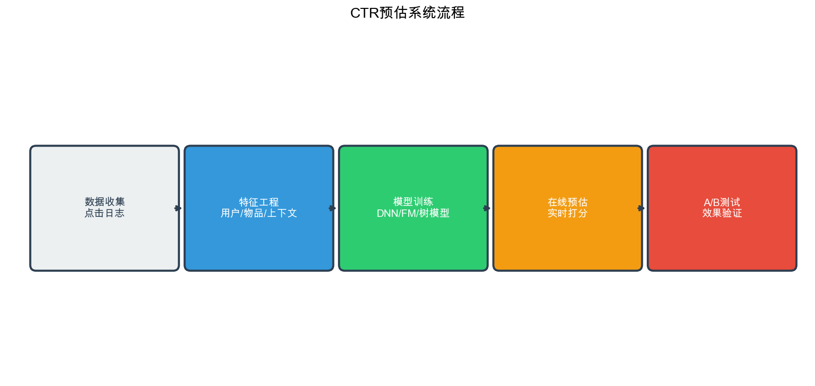
The CTR Prediction Pipeline

A typical CTR prediction pipeline consists of:

1
Raw Data → Feature Engineering → Feature Encoding → Model Training → Model Serving

Feature Engineering: - Extract features from user behavior, item attributes, context - Create interaction features (e.g., user_category combinations) - Handle missing values, outliers, normalization

Feature Encoding: - One-hot encoding for categorical features - Embedding layers for high-cardinality categorical features - Normalization for numerical features

Model Training: - Use appropriate loss function (binary cross-entropy) - Handle class imbalance (weighted loss, sampling) - Regularization to prevent overfitting

Model Serving: - Deploy model for real-time inference - Monitor performance metrics - A/B test new models

explore the evolution of CTR prediction models, starting with the simplest baseline.

Logistic Regression: The Foundation

Logistic Regression serves as the baseline for CTR prediction. Despite its simplicity, it's still widely used in production systems due to its interpretability, efficiency, and robustness.

Mathematical Formulation

Logistic Regression models the probability of a click as:\[P(y = 1 | \mathbf{x}) = \sigma(\mathbf{w}^T \mathbf{x} + b) = \frac{1}{1 + e^{-(\mathbf{w}^T \mathbf{x} + b) }}\]Where: -\(\mathbf{w} \in \mathbb{R}^d\)are the model weights -\(b \in \mathbb{R}\)is the bias term -\(\sigma(z) = \frac{1}{1 + e^{-z }}\)is the sigmoid function -\(\mathbf{x} \in \mathbb{R}^d\)is the feature vector

The sigmoid function maps the linear combination\(\mathbf{w}^T \mathbf{x} + b\)to a probability between 0 and 1.

Training Objective

We minimize the binary cross-entropy loss:\[\mathcal{L} = -\frac{1}{N} \sum_{i=1}^{N} \left[ y_i \log(\hat{y}_i) + (1 - y_i) \log(1 - \hat{y}_i) \right]\]Where\(\hat{y}_i = P(y_i = 1 | \mathbf{x}_i)\)is the predicted probability.

Implementation

Here's a complete implementation of Logistic Regression for CTR prediction:

1
2
3
4
5
6
7
8
9
10
11
12
13
14
15
16
17
18
19
20
21
22
23
24
25
26
27
28
29
30
31
32
33
34
35
36
37
38
39
40
41
42
43
44
45
46
47
48
49
50
51
52
53
54
55
56
57
58
59
60
61
62
63
64
65
66
67
68
69
70
71
72
73
74
75
76
77
78
79
80
import numpy as np
import torch
import torch.nn as nn
from sklearn.preprocessing import StandardScaler

class LogisticRegression(nn.Module):
"""
Logistic Regression model for CTR prediction.

Args:
input_dim: Dimension of input features
"""
def __init__(self, input_dim):
super(LogisticRegression, self).__init__()
self.linear = nn.Linear(input_dim, 1)

def forward(self, x):
"""
Forward pass.

Args:
x: Input features of shape (batch_size, input_dim)

Returns:
Predicted CTR probabilities of shape (batch_size, 1)
"""
return torch.sigmoid(self.linear(x))

# Example usage
def train_logistic_regression(X_train, y_train, X_val, y_val, epochs=100, lr=0.01):
"""
Train Logistic Regression model.

Args:
X_train: Training features (numpy array)
y_train: Training labels (numpy array)
X_val: Validation features (numpy array)
y_val: Validation labels (numpy array)
epochs: Number of training epochs
lr: Learning rate
"""
# Normalize features
scaler = StandardScaler()
X_train_scaled = scaler.fit_transform(X_train)
X_val_scaled = scaler.transform(X_val)

# Convert to tensors
X_train_tensor = torch.FloatTensor(X_train_scaled)
y_train_tensor = torch.FloatTensor(y_train).reshape(-1, 1)
X_val_tensor = torch.FloatTensor(X_val_scaled)
y_val_tensor = torch.FloatTensor(y_val).reshape(-1, 1)

# Initialize model
model = LogisticRegression(input_dim=X_train.shape[1])
criterion = nn.BCELoss()
optimizer = torch.optim.Adam(model.parameters(), lr=lr)

# Training loop
for epoch in range(epochs):
model.train()
optimizer.zero_grad()

# Forward pass
predictions = model(X_train_tensor)
loss = criterion(predictions, y_train_tensor)

# Backward pass
loss.backward()
optimizer.step()

# Validation
if (epoch + 1) % 10 == 0:
model.eval()
with torch.no_grad():
val_predictions = model(X_val_tensor)
val_loss = criterion(val_predictions, y_val_tensor)
print(f"Epoch {epoch+1}/{epochs}, Train Loss: {loss.item():.4f}, "
f"Val Loss: {val_loss.item():.4f}")

return model, scaler

Limitations of Logistic Regression

While Logistic Regression is simple and effective, it has significant limitations:

  1. No Feature Interactions: It assumes features are independent. The model can't learn that "young users clicking on action movies" is different from the sum of "young users" and "action movies" effects.

  2. Manual Feature Engineering Required: To capture interactions, engineers must manually create interaction features (e.g., user_age × item_category), which is:

    • Time-consuming and error-prone
    • Doesn't scale to high-order interactions
    • May miss important interactions
  3. Linear Decision Boundary: The model can only learn linear relationships, limiting its expressiveness.

These limitations motivated the development of Factorization Machines, which automatically learn feature interactions.

Factorization Machines (FM): Learning Feature Interactions

Factorization Machines, introduced by Steffen Rendle in 2010, were a breakthrough in CTR prediction. They automatically model pairwise feature interactions without requiring manual feature engineering.

Intuition

The key insight of FM is to model interactions between features using factorized parameters. Instead of learning a separate weight\(w_{ij}\)for each pair of features\((i, j)\)(which would require\(O(d^2)\)parameters), FM learns a low-rank factorization:\[w_{ij} \approx \langle \mathbf{v}_i, \mathbf{v}_j \rangle = \sum_{f=1}^{k} v_{i,f} \cdot v_{j,f}\]Where: -\(\mathbf{v}_i \in \mathbb{R}^k\)is the embedding vector for feature\(i\) -\(k\)is the embedding dimension (typically 8-64) -\(\langle \cdot, \cdot \rangle\)denotes the dot product

This reduces the number of parameters from\(O(d^2)\)to\(O(d \cdot k)\), making FM scalable to high-dimensional sparse data.

Mathematical Formulation

The FM model prediction is:\[\hat{y}(\mathbf{x}) = w_0 + \sum_{i=1}^{d} w_i x_i + \sum_{i=1}^{d} \sum_{j=i+1}^{d} \langle \mathbf{v}_i, \mathbf{v}_j \rangle x_i x_j\]Where: -\(w_0\)is the global bias -\(w_i\)are the linear weights for individual features -\(\langle \mathbf{v}_i, \mathbf{v}_j \rangle x_i x_j\)models pairwise interactions

The interaction term can be computed efficiently in\(O(k \cdot d)\)time using:\[\sum_{i=1}^{d} \sum_{j=i+1}^{d} \langle \mathbf{v}_i, \mathbf{v}_j \rangle x_i x_j = \frac{1}{2} \left[ \left( \sum_{i=1}^{d} \mathbf{v}_i x_i \right)^2 - \sum_{i=1}^{d} (\mathbf{v}_i x_i)^2 \right]\]This reformulation avoids the nested loop and makes FM computationally efficient.

Implementation

Here's a complete implementation of Factorization Machines:

1
2
3
4
5
6
7
8
9
10
11
12
13
14
15
16
17
18
19
20
21
22
23
24
25
26
27
28
29
30
31
32
33
34
35
36
37
38
39
40
41
42
43
44
45
46
47
48
49
50
51
52
53
54
55
56
57
58
59
60
61
62
63
64
65
66
67
68
69
70
71
72
73
74
75
76
77
78
79
80
81
82
83
84
85
86
87
88
89
90
91
92
93
94
95
96
97
98
99
100
101
102
103
104
105
106
107
108
109
110
111
112
113
114
115
116
117
118
119
120
121
122
123
124
125
126
127
128
129
130
131
import torch
import torch.nn as nn
import torch.nn.functional as F

class FactorizationMachine(nn.Module):
"""
Factorization Machine model for CTR prediction.

Args:
field_dims: List of sizes for each categorical field
embed_dim: Dimension of embedding vectors
"""
def __init__(self, field_dims, embed_dim=16):
super(FactorizationMachine, self).__init__()
self.field_dims = field_dims
self.embed_dim = embed_dim

# Linear part: bias + linear weights
self.linear = nn.Linear(sum(field_dims), 1)

# Embedding layer for feature interactions
self.embedding = nn.ModuleList([
nn.Embedding(field_dim, embed_dim) for field_dim in field_dims
])

def forward(self, x):
"""
Forward pass.

Args:
x: Input features of shape (batch_size, num_fields)
Each field is a categorical feature index

Returns:
Predicted CTR probabilities of shape (batch_size, 1)
"""
# Linear part
x_onehot = self._one_hot_encode(x)
linear_output = self.linear(x_onehot)

# Interaction part
# Get embeddings for each field
embeddings = [self.embedding[i](x[:, i]) for i in range(len(self.field_dims))]
embeddings = torch.stack(embeddings, dim=1) # (batch_size, num_fields, embed_dim)

# Compute pairwise interactions efficiently
# Sum of squares
sum_square = torch.sum(embeddings, dim=1) ** 2 # (batch_size, embed_dim)
# Square of sums
square_sum = torch.sum(embeddings ** 2, dim=1) # (batch_size, embed_dim)

# Interaction term
interaction = 0.5 * (sum_square - square_sum).sum(dim=1, keepdim=True)

# Combine linear and interaction parts
output = linear_output + interaction
return torch.sigmoid(output)

def _one_hot_encode(self, x):
"""Convert categorical indices to one-hot encoding."""
batch_size = x.size(0)
one_hot = torch.zeros(batch_size, sum(self.field_dims), device=x.device)
offset = 0
for i, field_dim in enumerate(self.field_dims):
one_hot.scatter_(1, x[:, i:i+1] + offset, 1)
offset += field_dim
return one_hot

# Example usage
def create_fm_example():
"""Example of using Factorization Machine."""
# Example: 3 categorical fields with sizes 10, 20, 15
field_dims = [10, 20, 15]
model = FactorizationMachine(field_dims, embed_dim=16)

# Example input: batch of 4 samples
# Each sample has 3 categorical features
x = torch.LongTensor([
[0, 5, 2], # Sample 1
[3, 10, 8], # Sample 2
[1, 7, 1], # Sample 3
[9, 15, 12] # Sample 4
])

predictions = model(x)
print(f"Predictions shape: {predictions.shape}")
print(f"Sample predictions: {predictions.squeeze()}")

return model

# Training function
def train_fm(model, train_loader, val_loader, epochs=100, lr=0.001):
"""
Train Factorization Machine model.

Args:
model: FM model instance
train_loader: Training data loader
val_loader: Validation data loader
epochs: Number of training epochs
lr: Learning rate
"""
criterion = nn.BCELoss()
optimizer = torch.optim.Adam(model.parameters(), lr=lr)

for epoch in range(epochs):
# Training
model.train()
train_loss = 0.0
for batch_x, batch_y in train_loader:
optimizer.zero_grad()
predictions = model(batch_x).squeeze()
loss = criterion(predictions, batch_y)
loss.backward()
optimizer.step()
train_loss += loss.item()

# Validation
if (epoch + 1) % 10 == 0:
model.eval()
val_loss = 0.0
with torch.no_grad():
for batch_x, batch_y in val_loader:
predictions = model(batch_x).squeeze()
loss = criterion(predictions, batch_y)
val_loss += loss.item()

print(f"Epoch {epoch+1}/{epochs}, Train Loss: {train_loss/len(train_loader):.4f}, "
f"Val Loss: {val_loss/len(val_loader):.4f}")

return model

Advantages of FM

  1. Automatic Feature Interactions: Learns pairwise interactions without manual engineering

  2. Scalability:\(O(k \cdot d)\)complexity instead of\(O(d^2)\)

  3. Sparse Data Handling: Works well with high-dimensional sparse features

  4. Interpretability: Can analyze learned embeddings to understand feature relationships

Limitations

  1. Only Pairwise Interactions: Cannot model higher-order interactions (3-way, 4-way, etc.)
  2. Same Embedding for All Interactions: All features share the same embedding space, which may not be optimal

These limitations led to the development of Field-aware Factorization Machines.

Field-aware Factorization Machines (FFM)

Field-aware Factorization Machines extend FM by introducing the concept of "fields." A field is a group of related features (e.g., all user-related features form one field, all item-related features form another).

Key Innovation

In FFM, each feature has multiple embedding vectors, one for each field it interacts with. This allows the model to learn field-specific interaction patterns.

Mathematical Formulation

The FFM prediction is:\[\hat{y}(\mathbf{x}) = w_0 + \sum_{i=1}^{d} w_i x_i + \sum_{i=1}^{d} \sum_{j=i+1}^{d} \langle \mathbf{v}_{i, f_j}, \mathbf{v}_{j, f_i} \rangle x_i x_j\]Where: -\(f_i\)is the field that feature\(i\)belongs to -\(\mathbf{v}_{i, f_j}\)is the embedding vector of feature\(i\)when interacting with field\(f_j\)The key difference from FM is that\(\mathbf{v}_{i, f_j} \ne \mathbf{v}_{i, f_k}\)for\(j \ne k\)– each feature has different embeddings for different fields.

Implementation

1
2
3
4
5
6
7
8
9
10
11
12
13
14
15
16
17
18
19
20
21
22
23
24
25
26
27
28
29
30
31
32
33
34
35
36
37
38
39
40
41
42
43
44
45
46
47
48
49
50
51
52
53
54
55
56
57
58
59
60
61
62
63
64
65
66
67
68
69
70
71
72
73
74
75
76
77
78
79
80
81
82
83
84
85
86
87
88
89
90
class FieldAwareFactorizationMachine(nn.Module):
"""
Field-aware Factorization Machine model.

Args:
field_dims: List of sizes for each categorical field
num_fields: Number of distinct fields
embed_dim: Dimension of embedding vectors
"""
def __init__(self, field_dims, num_fields, embed_dim=16):
super(FieldAwareFactorizationMachine, self).__init__()
self.field_dims = field_dims
self.num_fields = num_fields
self.embed_dim = embed_dim

# Linear part
self.linear = nn.Linear(sum(field_dims), 1)

# Field-aware embeddings
# Each feature has num_fields embeddings (one for each field)
self.embeddings = nn.ModuleList([
nn.ModuleList([
nn.Embedding(field_dim, embed_dim)
for _ in range(num_fields)
]) for field_dim in field_dims
])

# Field mapping: which field does each feature belong to?
self.field_map = self._create_field_map()

def _create_field_map(self):
"""Create mapping from feature index to field index."""
field_map = []
for field_idx, field_dim in enumerate(self.field_dims):
field_map.extend([field_idx] * field_dim)
return field_map

def forward(self, x):
"""
Forward pass.

Args:
x: Input features of shape (batch_size, num_fields)

Returns:
Predicted CTR probabilities of shape (batch_size, 1)
"""
batch_size = x.size(0)

# Linear part
x_onehot = self._one_hot_encode(x)
linear_output = self.linear(x_onehot)

# Field-aware interaction part
# Get embeddings for each field-feature pair
embeddings_list = []
for field_idx in range(len(self.field_dims)):
feature_idx = x[:, field_idx] # (batch_size,)
# Get embedding for this feature when interacting with each field
field_embeddings = []
for target_field_idx in range(self.num_fields):
emb = self.embeddings[field_idx][target_field_idx](feature_idx)
field_embeddings.append(emb)
embeddings_list.append(torch.stack(field_embeddings, dim=1))
# Shape: (batch_size, num_fields, embed_dim)

# Compute interactions
interaction_sum = 0.0
for i in range(len(self.field_dims)):
for j in range(i + 1, len(self.field_dims)):
# Feature i interacting with field j
v_i_fj = embeddings_list[i][:, j, :] # (batch_size, embed_dim)
# Feature j interacting with field i
v_j_fi = embeddings_list[j][:, i, :] # (batch_size, embed_dim)
# Interaction
interaction = (v_i_fj * v_j_fi).sum(dim=1, keepdim=True)
interaction_sum += interaction

output = linear_output + interaction_sum
return torch.sigmoid(output)

def _one_hot_encode(self, x):
"""Convert categorical indices to one-hot encoding."""
batch_size = x.size(0)
one_hot = torch.zeros(batch_size, sum(self.field_dims), device=x.device)
offset = 0
for i, field_dim in enumerate(self.field_dims):
one_hot.scatter_(1, x[:, i:i+1] + offset, 1)
offset += field_dim
return one_hot

FFM vs FM

FFM Advantages: - More expressive: Field-specific embeddings capture domain knowledge - Better performance on datasets with clear field structure

FFM Disadvantages: - More parameters:\(O(d \cdot F \cdot k)\)vs\(O(d \cdot k)\)where\(F\)is number of fields - More complex: Harder to train and tune - Field definition required: Need domain knowledge to define fields

In practice, FFM often performs better than FM but requires more careful tuning. However, both FM and FFM are limited to pairwise interactions. The next generation of models uses deep learning to automatically learn higher-order interactions.

DeepFM: Combining Factorization Machines with Deep Learning

DeepFM, introduced by Huawei in 2017, combines the strengths of Factorization Machines (for low-order interactions) with deep neural networks (for high-order interactions). It's one of the most widely used CTR prediction models in industry.

Architecture Overview

DeepFM consists of two components:

  1. FM Component: Models low-order (especially pairwise) feature interactions
  2. Deep Component: A multi-layer neural network that models high-order feature interactions

Both components share the same embedding layer, which reduces model complexity and improves training efficiency.

Mathematical Formulation

The DeepFM prediction is:\[\hat{y}(\mathbf{x}) = \sigma(y_{FM} + y_{Deep})\]Where: -\(y_{FM}\)is the FM component output (same as standard FM) -\(y_{Deep}\)is the deep component output -\(\sigma\)is the sigmoid function

The deep component processes the concatenated embeddings through multiple fully-connected layers:\[\mathbf{h}_0 = [\mathbf{v}_1, \mathbf{v}_2, \ldots, \mathbf{v}_d]\] \[\mathbf{h}_l = \text{ReLU}(\mathbf{W}_l \mathbf{h}_{l-1} + \mathbf{b}_l), \quad l = 1, 2, \ldots, L\] \[y_{Deep} = \mathbf{W}_{L+1} \mathbf{h}_L + b_{L+1}\]

Implementation

Here's a complete implementation of DeepFM:

1
2
3
4
5
6
7
8
9
10
11
12
13
14
15
16
17
18
19
20
21
22
23
24
25
26
27
28
29
30
31
32
33
34
35
36
37
38
39
40
41
42
43
44
45
46
47
48
49
50
51
52
53
54
55
56
57
58
59
60
61
62
63
64
65
66
67
68
69
70
71
72
73
74
75
76
77
78
79
80
81
82
83
84
85
86
87
88
89
90
91
92
93
94
95
96
97
98
99
100
101
102
103
class DeepFM(nn.Module):
"""
DeepFM model combining FM and Deep Neural Network.

Args:
field_dims: List of sizes for each categorical field
embed_dim: Dimension of embedding vectors
mlp_dims: List of dimensions for MLP layers
dropout: Dropout rate
"""
def __init__(self, field_dims, embed_dim=16, mlp_dims=[128, 64], dropout=0.2):
super(DeepFM, self).__init__()
self.field_dims = field_dims
self.embed_dim = embed_dim
self.num_fields = len(field_dims)

# Shared embedding layer
self.embedding = nn.ModuleList([
nn.Embedding(field_dim, embed_dim) for field_dim in field_dims
])

# FM component: linear + interaction
self.linear = nn.Linear(sum(field_dims), 1)

# Deep component: MLP
mlp_input_dim = self.num_fields * embed_dim
mlp_layers = []
prev_dim = mlp_input_dim
for mlp_dim in mlp_dims:
mlp_layers.append(nn.Linear(prev_dim, mlp_dim))
mlp_layers.append(nn.BatchNorm1d(mlp_dim))
mlp_layers.append(nn.ReLU())
mlp_layers.append(nn.Dropout(dropout))
prev_dim = mlp_dim
mlp_layers.append(nn.Linear(prev_dim, 1))
self.mlp = nn.Sequential(*mlp_layers)

def forward(self, x):
"""
Forward pass.

Args:
x: Input features of shape (batch_size, num_fields)

Returns:
Predicted CTR probabilities of shape (batch_size, 1)
"""
# Get embeddings
embeddings = [self.embedding[i](x[:, i]) for i in range(self.num_fields)]
embeddings = torch.stack(embeddings, dim=1) # (batch_size, num_fields, embed_dim)

# FM component
# Linear part
x_onehot = self._one_hot_encode(x)
fm_linear = self.linear(x_onehot)

# Interaction part
sum_square = torch.sum(embeddings, dim=1) ** 2
square_sum = torch.sum(embeddings ** 2, dim=1)
fm_interaction = 0.5 * (sum_square - square_sum).sum(dim=1, keepdim=True)
fm_output = fm_linear + fm_interaction

# Deep component
deep_input = embeddings.view(embeddings.size(0), -1) # Flatten
deep_output = self.mlp(deep_input)

# Combine FM and Deep
output = fm_output + deep_output
return torch.sigmoid(output)

def _one_hot_encode(self, x):
"""Convert categorical indices to one-hot encoding."""
batch_size = x.size(0)
one_hot = torch.zeros(batch_size, sum(self.field_dims), device=x.device)
offset = 0
for i, field_dim in enumerate(self.field_dims):
one_hot.scatter_(1, x[:, i:i+1] + offset, 1)
offset += field_dim
return one_hot

# Example usage
def create_deepfm_example():
"""Example of using DeepFM."""
field_dims = [10, 20, 15, 30] # 4 categorical fields
model = DeepFM(
field_dims=field_dims,
embed_dim=16,
mlp_dims=[128, 64, 32],
dropout=0.2
)

# Example input
x = torch.LongTensor([
[0, 5, 2, 10],
[3, 10, 8, 20],
[1, 7, 1, 5],
[9, 15, 12, 25]
])

predictions = model(x)
print(f"DeepFM predictions: {predictions.squeeze()}")

return model

Why DeepFM Works

  1. Complementary Strengths: FM captures low-order interactions explicitly, while the deep network captures high-order interactions implicitly
  2. Shared Embeddings: Reduces parameters and improves training stability
  3. End-to-End Learning: Both components are trained jointly, allowing them to complement each other

DeepFM has become a standard baseline in CTR prediction competitions and production systems. However, researchers noticed that the deep component's ability to learn feature interactions might be limited. This led to the development of xDeepFM, which explicitly models feature interactions in the deep component.

xDeepFM: Explicit High-Order Feature Interactions

xDeepFM (eXtreme Deep Factorization Machine) addresses a key limitation of DeepFM: while the deep network can theoretically learn high-order interactions, it doesn't explicitly model them. xDeepFM introduces the Compressed Interaction Network (CIN) to explicitly learn high-order feature interactions.

Key Innovation: Compressed Interaction Network (CIN)

CIN explicitly models feature interactions at each layer, similar to how CNNs learn spatial patterns in images. At each layer, CIN: 1. Computes interactions between the current layer's features and the original embeddings 2. Compresses the interaction results to a fixed dimension 3. Passes the compressed interactions to the next layer

Mathematical Formulation

Let\(\mathbf{X}^0 \in \mathbb{R}^{m \times D}\)be the embedding matrix where\(m\)is the number of fields and\(D\)is the embedding dimension. The\(k\)-th layer of CIN computes:\[\mathbf{X}^k_{h,*} = \sum_{i=1}^{H_{k-1 }} \sum_{j=1}^{m} \mathbf{W}^{k,h}_{i,j} (\mathbf{X}^{k-1}_{i,*} \circ \mathbf{X}^0_{j,*})\]Where: -\(H_k\)is the number of feature maps in layer\(k\) -\(\circ\)denotes element-wise product (Hadamard product) -\(\mathbf{W}^{k,h}\)are learnable parameters

The final CIN output is the sum of all layers' outputs (after pooling):\[\mathbf{p}^+ = [\mathbf{p}^1, \mathbf{p}^2, \ldots, \mathbf{p}^H]\]Where\(\mathbf{p}^h\)is the sum-pooling of the\(h\)-th feature map.

Implementation

1
2
3
4
5
6
7
8
9
10
11
12
13
14
15
16
17
18
19
20
21
22
23
24
25
26
27
28
29
30
31
32
33
34
35
36
37
38
39
40
41
42
43
44
45
46
47
48
49
50
51
52
53
54
55
56
57
58
59
60
61
62
63
64
65
66
67
68
69
70
71
72
73
74
75
76
77
78
79
80
81
82
83
84
85
86
87
88
89
90
91
92
93
94
95
96
97
98
99
100
101
102
103
104
105
106
107
108
109
110
111
112
113
114
115
116
117
118
119
120
121
122
123
124
125
126
127
128
129
130
131
132
133
134
135
136
137
138
139
140
141
142
143
144
145
146
147
148
149
150
151
152
153
154
155
156
157
158
159
160
161
162
163
164
165
166
167
168
169
170
171
172
173
174
175
176
177
class CompressedInteractionNetwork(nn.Module):
"""
Compressed Interaction Network (CIN) for explicit feature interactions.

Args:
field_dims: List of sizes for each categorical field
embed_dim: Dimension of embedding vectors
cin_layer_sizes: List of feature map sizes for each CIN layer
"""
def __init__(self, field_dims, embed_dim, cin_layer_sizes=[100, 100]):
super(CompressedInteractionNetwork, self).__init__()
self.field_dims = field_dims
self.embed_dim = embed_dim
self.num_fields = len(field_dims)
self.cin_layer_sizes = cin_layer_sizes

# Embedding layer
self.embedding = nn.ModuleList([
nn.Embedding(field_dim, embed_dim) for field_dim in field_dims
])

# CIN layers
self.cin_layers = nn.ModuleList()
prev_size = self.num_fields
for layer_size in cin_layer_sizes:
# Each layer learns interactions with original embeddings
cin_layer = nn.Conv1d(
in_channels=prev_size * self.num_fields,
out_channels=layer_size,
kernel_size=1,
groups=prev_size
)
self.cin_layers.append(cin_layer)
prev_size = layer_size

def forward(self, x):
"""
Forward pass through CIN.

Args:
x: Input features of shape (batch_size, num_fields)

Returns:
CIN output of shape (batch_size, sum(cin_layer_sizes))
"""
batch_size = x.size(0)

# Get embeddings: (batch_size, num_fields, embed_dim)
embeddings = torch.stack([
self.embedding[i](x[:, i]) for i in range(self.num_fields)
], dim=1)

# X^0: original embeddings
X_0 = embeddings # (batch_size, num_fields, embed_dim)
X_k = X_0 # Current layer

cin_outputs = []

for cin_layer in self.cin_layers:
# Compute interactions: (X^{k-1}, X^0) -> X^k
# X^{k-1}: (batch_size, H_{k-1}, embed_dim)
# X^0: (batch_size, num_fields, embed_dim)

# Outer product and reshape for convolution
# We need to compute interactions between each feature map in X_k
# and each field in X_0
H_k_minus_1 = X_k.size(1)

# Expand dimensions for broadcasting
X_k_expanded = X_k.unsqueeze(2) # (batch_size, H_{k-1}, 1, embed_dim)
X_0_expanded = X_0.unsqueeze(1) # (batch_size, 1, num_fields, embed_dim)

# Element-wise product: (batch_size, H_{k-1}, num_fields, embed_dim)
interactions = X_k_expanded * X_0_expanded

# Reshape for convolution: (batch_size, H_{k-1} * num_fields, embed_dim)
interactions = interactions.view(batch_size, H_k_minus_1 * self.num_fields, self.embed_dim)

# Apply 1D convolution (acts as weighted sum)
X_k = cin_layer(interactions) # (batch_size, layer_size, embed_dim)
X_k = F.relu(X_k)

# Sum pooling over embedding dimension
p_k = X_k.sum(dim=2) # (batch_size, layer_size)
cin_outputs.append(p_k)

# Concatenate all layer outputs
cin_output = torch.cat(cin_outputs, dim=1) # (batch_size, sum(cin_layer_sizes))
return cin_output


class xDeepFM(nn.Module):
"""
xDeepFM model with CIN for explicit high-order interactions.

Args:
field_dims: List of sizes for each categorical field
embed_dim: Dimension of embedding vectors
cin_layer_sizes: List of feature map sizes for CIN layers
mlp_dims: List of dimensions for MLP layers
dropout: Dropout rate
"""
def __init__(self, field_dims, embed_dim=16, cin_layer_sizes=[100, 100],
mlp_dims=[128, 64], dropout=0.2):
super(xDeepFM, self).__init__()
self.field_dims = field_dims
self.embed_dim = embed_dim
self.num_fields = len(field_dims)

# Shared embedding layer
self.embedding = nn.ModuleList([
nn.Embedding(field_dim, embed_dim) for field_dim in field_dims
])

# Linear component
self.linear = nn.Linear(sum(field_dims), 1)

# CIN component
self.cin = CompressedInteractionNetwork(
field_dims, embed_dim, cin_layer_sizes
)
cin_output_dim = sum(cin_layer_sizes)

# Deep component (MLP)
mlp_input_dim = self.num_fields * embed_dim
mlp_layers = []
prev_dim = mlp_input_dim
for mlp_dim in mlp_dims:
mlp_layers.append(nn.Linear(prev_dim, mlp_dim))
mlp_layers.append(nn.BatchNorm1d(mlp_dim))
mlp_layers.append(nn.ReLU())
mlp_layers.append(nn.Dropout(dropout))
prev_dim = mlp_dim
mlp_layers.append(nn.Linear(prev_dim, 1))
self.mlp = nn.Sequential(*mlp_layers)

# Final projection for CIN output
self.cin_projection = nn.Linear(cin_output_dim, 1)

def forward(self, x):
"""
Forward pass.

Args:
x: Input features of shape (batch_size, num_fields)

Returns:
Predicted CTR probabilities of shape (batch_size, 1)
"""
# Linear part
x_onehot = self._one_hot_encode(x)
linear_output = self.linear(x_onehot)

# CIN part
cin_output = self.cin(x)
cin_projection = self.cin_projection(cin_output)

# Deep part
embeddings = torch.stack([
self.embedding[i](x[:, i]) for i in range(self.num_fields)
], dim=1)
deep_input = embeddings.view(embeddings.size(0), -1)
deep_output = self.mlp(deep_input)

# Combine all components
output = linear_output + cin_projection + deep_output
return torch.sigmoid(output)

def _one_hot_encode(self, x):
"""Convert categorical indices to one-hot encoding."""
batch_size = x.size(0)
one_hot = torch.zeros(batch_size, sum(self.field_dims), device=x.device)
offset = 0
for i, field_dim in enumerate(self.field_dims):
one_hot.scatter_(1, x[:, i:i+1] + offset, 1)
offset += field_dim
return one_hot

xDeepFM vs DeepFM

xDeepFM Advantages: - Explicit high-order interactions through CIN - Better interpretability (can analyze CIN layers) - Often achieves better performance on complex datasets

xDeepFM Disadvantages: - More complex architecture - Higher computational cost (CIN layers) - More hyperparameters to tune

xDeepFM represents a significant advancement in explicitly modeling feature interactions. However, another important direction in CTR prediction is learning cross-features automatically, which is the focus of DCN.

Deep & Cross Network (DCN): Learning Cross-Features Automatically

The Deep & Cross Network (DCN), introduced by Google in 2017, addresses feature interaction learning from a different angle. Instead of using factorization machines or CIN, DCN uses a "cross network" that explicitly learns bounded-degree feature interactions.

Architecture Overview

DCN consists of two components:

  1. Cross Network: Learns explicit feature interactions of bounded degree
  2. Deep Network: Standard MLP for implicit high-order interactions

The outputs of both networks are combined for the final prediction.

Cross Network Formulation

The cross network applies the following transformation at each layer:\[\mathbf{x}_{l+1} = \mathbf{x}_0 \mathbf{x}_l^T \mathbf{w}_l + \mathbf{b}_l + \mathbf{x}_l\]Where: -\(\mathbf{x}_0\)is the input embedding -\(\mathbf{x}_l\)is the output of layer\(l\) -\(\mathbf{w}_l, \mathbf{b}_l\)are learnable parameters

The key insight is that each cross layer increases the polynomial degree of interactions by 1. After\(L\)layers, the model can learn interactions up to degree\(L+1\).

Implementation

1
2
3
4
5
6
7
8
9
10
11
12
13
14
15
16
17
18
19
20
21
22
23
24
25
26
27
28
29
30
31
32
33
34
35
36
37
38
39
40
41
42
43
44
45
46
47
48
49
50
51
52
53
54
55
56
57
58
59
60
61
62
63
64
65
66
67
68
69
70
71
72
73
74
75
76
77
78
79
80
81
82
83
84
85
86
87
88
89
90
91
92
93
94
95
96
97
98
99
100
101
102
103
104
105
106
107
108
109
110
class CrossNetwork(nn.Module):
"""
Cross Network for explicit feature interactions.

Args:
input_dim: Input dimension
num_layers: Number of cross layers
"""
def __init__(self, input_dim, num_layers=3):
super(CrossNetwork, self).__init__()
self.num_layers = num_layers
self.cross_layers = nn.ModuleList([
nn.Linear(input_dim, 1, bias=True) for _ in range(num_layers)
])

def forward(self, x):
"""
Forward pass.

Args:
x: Input of shape (batch_size, input_dim)

Returns:
Output of shape (batch_size, input_dim)
"""
x_0 = x
x_l = x

for i, cross_layer in enumerate(self.cross_layers):
# x_0^T * x_l (element-wise, then weighted sum)
# We compute this efficiently using the linear layer
# The linear layer learns: w^T * (x_0 * x_l) + b
x_l_w = cross_layer(x_l) # (batch_size, 1)
x_l_cross = x_0 * x_l_w # (batch_size, input_dim)
x_l = x_l_cross + x_l # Residual connection

return x_l


class DeepCrossNetwork(nn.Module):
"""
Deep & Cross Network (DCN) model.

Args:
field_dims: List of sizes for each categorical field
embed_dim: Dimension of embedding vectors
cross_num_layers: Number of cross network layers
mlp_dims: List of dimensions for MLP layers
dropout: Dropout rate
"""
def __init__(self, field_dims, embed_dim=16, cross_num_layers=3,
mlp_dims=[128, 64], dropout=0.2):
super(DeepCrossNetwork, self).__init__()
self.field_dims = field_dims
self.embed_dim = embed_dim
self.num_fields = len(field_dims)

# Embedding layer
self.embedding = nn.ModuleList([
nn.Embedding(field_dim, embed_dim) for field_dim in field_dims
])

# Input dimension for cross and deep networks
input_dim = self.num_fields * embed_dim

# Cross network
self.cross_net = CrossNetwork(input_dim, cross_num_layers)

# Deep network (MLP)
mlp_layers = []
prev_dim = input_dim
for mlp_dim in mlp_dims:
mlp_layers.append(nn.Linear(prev_dim, mlp_dim))
mlp_layers.append(nn.BatchNorm1d(mlp_dim))
mlp_layers.append(nn.ReLU())
mlp_layers.append(nn.Dropout(dropout))
prev_dim = mlp_dim
mlp_layers.append(nn.Linear(prev_dim, 1))
self.mlp = nn.Sequential(*mlp_layers)

# Final combination layer
self.final_layer = nn.Linear(input_dim + 1, 1)

def forward(self, x):
"""
Forward pass.

Args:
x: Input features of shape (batch_size, num_fields)

Returns:
Predicted CTR probabilities of shape (batch_size, 1)
"""
# Get embeddings and flatten
embeddings = torch.stack([
self.embedding[i](x[:, i]) for i in range(self.num_fields)
], dim=1)
embeddings_flat = embeddings.view(embeddings.size(0), -1)

# Cross network
cross_output = self.cross_net(embeddings_flat)

# Deep network
deep_output = self.mlp(embeddings_flat)

# Combine: concatenate cross output with deep output, then project
combined = torch.cat([cross_output, deep_output], dim=1)
output = self.final_layer(combined)

return torch.sigmoid(output)

DCN Advantages

  1. Bounded Interaction Degree: The number of cross layers directly controls the maximum interaction degree, providing interpretability
  2. Efficient: Cross network is computationally efficient
  3. Automatic Feature Learning: Learns cross-features automatically without manual engineering

DCN has been successfully deployed in production at Google and other companies. However, another important direction is using attention mechanisms to automatically identify important feature interactions, which is the focus of AutoInt.

AutoInt: Automatic Feature Interaction Learning via Attention

AutoInt, introduced in 2019, uses multi-head self-attention to automatically identify and model important feature interactions. The key insight is that not all feature interactions are equally important, and attention mechanisms can learn to focus on the most relevant ones.

Key Innovation: Multi-Head Self-Attention for Features

AutoInt treats each feature's embedding as a "token" and uses self-attention to learn which features should interact. This allows the model to: 1. Automatically discover important feature interactions 2. Assign different importance weights to different interactions 3. Model complex interaction patterns

Mathematical Formulation

Given feature embeddings\(\mathbf{E} = [\mathbf{e}_1, \mathbf{e}_2, \ldots, \mathbf{e}_m] \in \mathbb{R}^{m \times d}\), where\(m\)is the number of fields and\(d\)is the embedding dimension, the multi-head self-attention computes:\[\text{Attention}(\mathbf{Q}, \mathbf{K}, \mathbf{V}) = \text{softmax}\left(\frac{\mathbf{Q}\mathbf{K}^T}{\sqrt{d_k }}\right)\mathbf{V}\]Where\(\mathbf{Q} = \mathbf{E}\mathbf{W}_Q\),\(\mathbf{K} = \mathbf{E}\mathbf{W}_K\),\(\mathbf{V} = \mathbf{E}\mathbf{W}_V\)are query, key, and value matrices.

For\(H\)attention heads:\[\text{MultiHead}(\mathbf{E}) = \text{Concat}(\text{head}_1, \ldots, \text{head}_H)\mathbf{W}^O\]Where each head computes attention independently.

Implementation

1
2
3
4
5
6
7
8
9
10
11
12
13
14
15
16
17
18
19
20
21
22
23
24
25
26
27
28
29
30
31
32
33
34
35
36
37
38
39
40
41
42
43
44
45
46
47
48
49
50
51
52
53
54
55
56
57
58
59
60
61
62
63
64
65
66
67
68
69
70
71
72
73
74
75
76
77
78
79
80
81
82
83
84
85
86
87
88
89
90
91
92
93
94
95
96
97
98
99
100
101
102
103
104
105
106
107
108
109
110
111
112
113
114
115
116
117
118
119
120
121
122
123
124
125
126
127
128
129
130
131
132
133
134
135
136
137
138
139
140
141
142
143
144
145
146
147
148
149
150
151
152
153
154
155
156
157
158
159
160
161
162
163
164
165
166
class MultiHeadSelfAttention(nn.Module):
"""
Multi-head self-attention for feature interaction learning.

Args:
embed_dim: Embedding dimension
num_heads: Number of attention heads
dropout: Dropout rate
"""
def __init__(self, embed_dim, num_heads=4, dropout=0.1):
super(MultiHeadSelfAttention, self).__init__()
assert embed_dim % num_heads == 0

self.embed_dim = embed_dim
self.num_heads = num_heads
self.head_dim = embed_dim // num_heads

# Query, Key, Value projections
self.W_q = nn.Linear(embed_dim, embed_dim)
self.W_k = nn.Linear(embed_dim, embed_dim)
self.W_v = nn.Linear(embed_dim, embed_dim)
self.W_o = nn.Linear(embed_dim, embed_dim)

self.dropout = nn.Dropout(dropout)
self.layer_norm = nn.LayerNorm(embed_dim)

def forward(self, x):
"""
Forward pass.

Args:
x: Input of shape (batch_size, num_fields, embed_dim)

Returns:
Output of shape (batch_size, num_fields, embed_dim)
"""
batch_size, num_fields, embed_dim = x.size()
residual = x

# Apply layer norm
x = self.layer_norm(x)

# Compute Q, K, V
Q = self.W_q(x) # (batch_size, num_fields, embed_dim)
K = self.W_k(x)
V = self.W_v(x)

# Reshape for multi-head attention
Q = Q.view(batch_size, num_fields, self.num_heads, self.head_dim).transpose(1, 2)
K = K.view(batch_size, num_fields, self.num_heads, self.head_dim).transpose(1, 2)
V = V.view(batch_size, num_fields, self.num_heads, self.head_dim).transpose(1, 2)
# Now shape: (batch_size, num_heads, num_fields, head_dim)

# Compute attention scores
scores = torch.matmul(Q, K.transpose(-2, -1)) / np.sqrt(self.head_dim)
# (batch_size, num_heads, num_fields, num_fields)

attn_weights = F.softmax(scores, dim=-1)
attn_weights = self.dropout(attn_weights)

# Apply attention to values
attn_output = torch.matmul(attn_weights, V)
# (batch_size, num_heads, num_fields, head_dim)

# Concatenate heads
attn_output = attn_output.transpose(1, 2).contiguous().view(
batch_size, num_fields, embed_dim
)

# Final projection
output = self.W_o(attn_output)
output = self.dropout(output)

# Residual connection
output = output + residual

return output


class AutoInt(nn.Module):
"""
AutoInt model using multi-head self-attention.

Args:
field_dims: List of sizes for each categorical field
embed_dim: Dimension of embedding vectors
num_attention_layers: Number of attention layers
num_heads: Number of attention heads
mlp_dims: List of dimensions for MLP layers
dropout: Dropout rate
"""
def __init__(self, field_dims, embed_dim=16, num_attention_layers=3,
num_heads=4, mlp_dims=[128, 64], dropout=0.2):
super(AutoInt, self).__init__()
self.field_dims = field_dims
self.embed_dim = embed_dim
self.num_fields = len(field_dims)

# Embedding layer
self.embedding = nn.ModuleList([
nn.Embedding(field_dim, embed_dim) for field_dim in field_dims
])

# Linear component
self.linear = nn.Linear(sum(field_dims), 1)

# Attention layers
self.attention_layers = nn.ModuleList([
MultiHeadSelfAttention(embed_dim, num_heads, dropout)
for _ in range(num_attention_layers)
])

# MLP for final prediction
mlp_input_dim = self.num_fields * embed_dim
mlp_layers = []
prev_dim = mlp_input_dim
for mlp_dim in mlp_dims:
mlp_layers.append(nn.Linear(prev_dim, mlp_dim))
mlp_layers.append(nn.BatchNorm1d(mlp_dim))
mlp_layers.append(nn.ReLU())
mlp_layers.append(nn.Dropout(dropout))
prev_dim = mlp_dim
mlp_layers.append(nn.Linear(prev_dim, 1))
self.mlp = nn.Sequential(*mlp_layers)

def forward(self, x):
"""
Forward pass.

Args:
x: Input features of shape (batch_size, num_fields)

Returns:
Predicted CTR probabilities of shape (batch_size, 1)
"""
# Linear part
x_onehot = self._one_hot_encode(x)
linear_output = self.linear(x_onehot)

# Get embeddings: (batch_size, num_fields, embed_dim)
embeddings = torch.stack([
self.embedding[i](x[:, i]) for i in range(self.num_fields)
], dim=1)

# Apply attention layers
attn_output = embeddings
for attention_layer in self.attention_layers:
attn_output = attention_layer(attn_output)

# Flatten and pass through MLP
attn_flat = attn_output.view(attn_output.size(0), -1)
mlp_output = self.mlp(attn_flat)

# Combine linear and MLP outputs
output = linear_output + mlp_output
return torch.sigmoid(output)

def _one_hot_encode(self, x):
"""Convert categorical indices to one-hot encoding."""
batch_size = x.size(0)
one_hot = torch.zeros(batch_size, sum(self.field_dims), device=x.device)
offset = 0
for i, field_dim in enumerate(self.field_dims):
one_hot.scatter_(1, x[:, i:i+1] + offset, 1)
offset += field_dim
return one_hot

AutoInt Advantages

  1. Automatic Interaction Discovery: Attention mechanism automatically identifies important feature interactions
  2. Interpretability: Attention weights show which feature interactions are important
  3. Flexibility: Can model complex, non-linear interaction patterns

AutoInt demonstrates the power of attention mechanisms in CTR prediction. However, another important direction is improving feature representation itself, which is the focus of FiBiNet.

FiBiNet: Feature Importance and Bilinear Feature Interaction Network

FiBiNet (Feature Importance and Bilinear feature Interaction NETwork), introduced in 2019, addresses two key aspects of CTR prediction: 1. Feature Importance: Not all features are equally important 2. Feature Interactions: How features interact matters

FiBiNet introduces SENet (Squeeze-and-Excitation Network) for feature importance learning and bilinear interaction for feature interaction modeling.

Key Components

1. SENet for Feature Importance

SENet learns to reweight features based on their importance:

  1. Squeeze: Global average pooling to get feature importance scores
  2. Excitation: Two-layer MLP to learn importance weights
  3. Reweight: Multiply original features by importance weights

2. Bilinear Interaction

Instead of simple element-wise product (like in FM), FiBiNet uses bilinear interaction:\[f_{Bilinear}(\mathbf{v}_i, \mathbf{v}_j) = \mathbf{v}_i^T \mathbf{W} \mathbf{v}_j\]Where\(\mathbf{W}\)is a learnable matrix. This is more expressive than element-wise product.

Implementation

1
2
3
4
5
6
7
8
9
10
11
12
13
14
15
16
17
18
19
20
21
22
23
24
25
26
27
28
29
30
31
32
33
34
35
36
37
38
39
40
41
42
43
44
45
46
47
48
49
50
51
52
53
54
55
56
57
58
59
60
61
62
63
64
65
66
67
68
69
70
71
72
73
74
75
76
77
78
79
80
81
82
83
84
85
86
87
88
89
90
91
92
93
94
95
96
97
98
99
100
101
102
103
104
105
106
107
108
109
110
111
112
113
114
115
116
117
118
119
120
121
122
123
124
125
126
127
128
129
130
131
132
133
134
135
136
137
138
139
140
141
142
143
144
145
146
147
148
149
150
151
152
153
154
155
156
157
158
159
160
161
162
163
164
165
166
167
168
169
170
171
172
173
174
175
176
177
178
179
180
181
182
183
184
185
186
187
188
189
190
191
192
193
194
class SENet(nn.Module):
"""
Squeeze-and-Excitation Network for feature importance learning.

Args:
num_fields: Number of feature fields
reduction_ratio: Reduction ratio for excitation network
"""
def __init__(self, num_fields, reduction_ratio=4):
super(SENet, self).__init__()
self.num_fields = num_fields
reduced_dim = max(1, num_fields // reduction_ratio)

self.excitation = nn.Sequential(
nn.Linear(num_fields, reduced_dim),
nn.ReLU(),
nn.Linear(reduced_dim, num_fields),
nn.Sigmoid()
)

def forward(self, x):
"""
Forward pass.

Args:
x: Input of shape (batch_size, num_fields, embed_dim)

Returns:
Reweighted features of shape (batch_size, num_fields, embed_dim)
"""
# Squeeze: average pooling over embedding dimension
z = x.mean(dim=2) # (batch_size, num_fields)

# Excitation: learn importance weights
weights = self.excitation(z) # (batch_size, num_fields)

# Reweight: multiply by importance weights
weights = weights.unsqueeze(2) # (batch_size, num_fields, 1)
output = x * weights

return output


class BilinearInteraction(nn.Module):
"""
Bilinear feature interaction layer.

Args:
embed_dim: Embedding dimension
bilinear_type: Type of bilinear interaction ('field_all', 'field_each', 'field_interaction')
"""
def __init__(self, embed_dim, bilinear_type='field_all'):
super(BilinearInteraction, self).__init__()
self.embed_dim = embed_dim
self.bilinear_type = bilinear_type

if bilinear_type == 'field_all':
# Shared weight matrix for all field pairs
self.W = nn.Parameter(torch.randn(embed_dim, embed_dim))
elif bilinear_type == 'field_each':
# Separate weight matrix for each field
# This would require knowing num_fields, so we'll handle it differently
self.W = None # Will be set in forward
else: # field_interaction
# Separate weight matrix for each field pair
# This also requires num_fields
self.W = None

def forward(self, x, num_fields=None):
"""
Forward pass.

Args:
x: Input of shape (batch_size, num_fields, embed_dim)
num_fields: Number of fields (required for field_each and field_interaction)

Returns:
Interaction features of shape (batch_size, num_fields*(num_fields-1)//2, embed_dim)
"""
batch_size, n_fields, embed_dim = x.size()

if self.bilinear_type == 'field_all':
# Shared weight matrix
interactions = []
for i in range(n_fields):
for j in range(i + 1, n_fields):
# Bilinear: v_i^T W v_j
interaction = torch.matmul(x[:, i:i+1, :], self.W) # (batch_size, 1, embed_dim)
interaction = torch.matmul(interaction, x[:, j:j+1, :].transpose(1, 2))
interaction = interaction.squeeze(2) # (batch_size, embed_dim)
interactions.append(interaction)

output = torch.stack(interactions, dim=1) # (batch_size, num_interactions, embed_dim)
return output
else:
# For simplicity, we'll use field_all in this implementation
# Full implementation would handle field_each and field_interaction
return self.forward(x)


class FiBiNet(nn.Module):
"""
FiBiNet: Feature Importance and Bilinear feature Interaction NETwork.

Args:
field_dims: List of sizes for each categorical field
embed_dim: Dimension of embedding vectors
bilinear_type: Type of bilinear interaction
mlp_dims: List of dimensions for MLP layers
dropout: Dropout rate
"""
def __init__(self, field_dims, embed_dim=16, bilinear_type='field_all',
mlp_dims=[128, 64], dropout=0.2):
super(FiBiNet, self).__init__()
self.field_dims = field_dims
self.embed_dim = embed_dim
self.num_fields = len(field_dims)

# Embedding layer
self.embedding = nn.ModuleList([
nn.Embedding(field_dim, embed_dim) for field_dim in field_dims
])

# Linear component
self.linear = nn.Linear(sum(field_dims), 1)

# SENet for feature importance
self.senet = SENet(self.num_fields)

# Bilinear interaction
self.bilinear = BilinearInteraction(embed_dim, bilinear_type)

# MLP for final prediction
# Input: original embeddings + SENet embeddings + bilinear interactions
num_interactions = self.num_fields * (self.num_fields - 1) // 2
mlp_input_dim = self.num_fields * embed_dim * 2 + num_interactions * embed_dim

mlp_layers = []
prev_dim = mlp_input_dim
for mlp_dim in mlp_dims:
mlp_layers.append(nn.Linear(prev_dim, mlp_dim))
mlp_layers.append(nn.BatchNorm1d(mlp_dim))
mlp_layers.append(nn.ReLU())
mlp_layers.append(nn.Dropout(dropout))
prev_dim = mlp_dim
mlp_layers.append(nn.Linear(prev_dim, 1))
self.mlp = nn.Sequential(*mlp_layers)

def forward(self, x):
"""
Forward pass.

Args:
x: Input features of shape (batch_size, num_fields)

Returns:
Predicted CTR probabilities of shape (batch_size, 1)
"""
# Linear part
x_onehot = self._one_hot_encode(x)
linear_output = self.linear(x_onehot)

# Get embeddings: (batch_size, num_fields, embed_dim)
embeddings = torch.stack([
self.embedding[i](x[:, i]) for i in range(self.num_fields)
], dim=1)

# SENet: learn feature importance and reweight
senet_embeddings = self.senet(embeddings)

# Bilinear interactions on original embeddings
bilinear_interactions = self.bilinear(embeddings, self.num_fields)

# Concatenate: original + SENet + bilinear interactions
original_flat = embeddings.view(embeddings.size(0), -1)
senet_flat = senet_embeddings.view(senet_embeddings.size(0), -1)
bilinear_flat = bilinear_interactions.view(bilinear_interactions.size(0), -1)

mlp_input = torch.cat([original_flat, senet_flat, bilinear_flat], dim=1)
mlp_output = self.mlp(mlp_input)

# Combine linear and MLP outputs
output = linear_output + mlp_output
return torch.sigmoid(output)

def _one_hot_encode(self, x):
"""Convert categorical indices to one-hot encoding."""
batch_size = x.size(0)
one_hot = torch.zeros(batch_size, sum(self.field_dims), device=x.device)
offset = 0
for i, field_dim in enumerate(self.field_dims):
one_hot.scatter_(1, x[:, i:i+1] + offset, 1)
offset += field_dim
return one_hot

FiBiNet Advantages

  1. Feature Importance Learning: SENet automatically identifies important features
  2. Expressive Interactions: Bilinear interactions are more expressive than element-wise products
  3. Interpretability: Can analyze SENet weights to understand feature importance

FiBiNet demonstrates how improving feature representation can lead to better CTR prediction performance.

Model Comparison and Selection

Now that we've covered the major CTR prediction models, let's compare them across different dimensions:

Computational Complexity

Model Parameters Training Time Inference Time
LR \(O(d)\) Fast Very Fast
FM \(O(d \cdot k)\) Fast Fast
FFM \(O(d \cdot F \cdot k)\) Medium Medium
DeepFM \(O(d \cdot k + MLP)\) Medium Medium
xDeepFM \(O(d \cdot k + CIN + MLP)\) Slow Medium
DCN \(O(d \cdot k + Cross + MLP)\) Medium Medium
AutoInt \(O(d \cdot k + Attention + MLP)\) Medium Medium
FiBiNet \(O(d \cdot k + SENet + Bilinear + MLP)\) Medium Medium

Interaction Modeling Capability

Model Low-Order High-Order Explicit Implicit
LR Linear only No No No
FM Pairwise No Yes No
FFM Pairwise (field-aware) No Yes No
DeepFM Pairwise Yes Yes Yes
xDeepFM Pairwise Yes (bounded) Yes Yes
DCN Bounded degree Yes Yes Yes
AutoInt All orders Yes Yes (via attention) Yes
FiBiNet Pairwise (bilinear) Yes Yes Yes

When to Use Which Model?

Logistic Regression: - Baseline for comparison - When interpretability is critical - When data is very limited - When latency requirements are extreme

FM/FFM: - When you need explicit pairwise interactions - When computational resources are limited - When you have domain knowledge about fields (FFM)

DeepFM: - General-purpose choice for most scenarios - Good balance of performance and complexity - When you need both low-order and high-order interactions

xDeepFM: - When you need explicit high-order interactions - When interpretability of interactions matters - When you have sufficient computational resources

DCN: - When you want bounded interaction degree - When you need automatic cross-feature learning - Google-style production systems

AutoInt: - When you want automatic interaction discovery - When interpretability of attention weights is useful - When feature interactions are complex and non-linear

FiBiNet: - When feature importance varies significantly - When you need more expressive interactions than FM - When you want to understand which features matter

Training Strategies and Best Practices

Implementing the models is only half the battle. Here are essential training strategies for CTR prediction:

Handling Class Imbalance

CTR prediction suffers from extreme class imbalance. Here are effective strategies:

1. Weighted Loss Function

1
2
3
4
5
6
7
8
9
10
11
12
13
14
15
16
def weighted_bce_loss(predictions, targets, pos_weight):
"""
Weighted binary cross-entropy loss.

Args:
predictions: Predicted probabilities
targets: True labels
pos_weight: Weight for positive class
"""
loss = -pos_weight * targets * torch.log(predictions + 1e-8) - \
(1 - targets) * torch.log(1 - predictions + 1e-8)
return loss.mean()

# Usage: pos_weight = num_negatives / num_positives
pos_weight = torch.tensor([num_negatives / num_positives])
criterion = nn.BCEWithLogitsLoss(pos_weight=pos_weight)

2. Negative Sampling

Instead of using all negative examples, sample a subset:

1
2
3
4
5
6
7
8
9
10
11
12
13
14
15
16
17
18
19
20
def sample_negatives(positive_samples, num_negatives_per_positive, item_pool):
"""
Sample negative examples for each positive example.

Args:
positive_samples: List of (user_id, item_id) tuples
num_negatives_per_positive: Number of negatives per positive
item_pool: Set of all possible items
"""
negative_samples = []
for user_id, pos_item_id in positive_samples:
# Sample items that user hasn't interacted with
user_items = set(get_user_items(user_id))
candidate_items = item_pool - user_items

negatives = random.sample(candidate_items, num_negatives_per_positive)
for neg_item_id in negatives:
negative_samples.append((user_id, neg_item_id, 0))

return negative_samples

3. Focal Loss

Focal loss downweights easy examples and focuses on hard examples:

1
2
3
4
5
6
7
8
9
10
11
12
13
14
15
16
17
18
class FocalLoss(nn.Module):
"""
Focal Loss for addressing class imbalance.

Args:
alpha: Weighting factor for rare class
gamma: Focusing parameter
"""
def __init__(self, alpha=1.0, gamma=2.0):
super(FocalLoss, self).__init__()
self.alpha = alpha
self.gamma = gamma

def forward(self, predictions, targets):
bce_loss = F.binary_cross_entropy(predictions, targets, reduction='none')
pt = torch.where(targets == 1, predictions, 1 - predictions)
focal_loss = self.alpha * (1 - pt) ** self.gamma * bce_loss
return focal_loss.mean()

Feature Engineering

1. Categorical Feature Encoding

1
2
3
4
5
6
7
8
9
10
11
12
13
14
15
16
17
18
19
def encode_categorical_features(df, categorical_columns):
"""
Encode categorical features using label encoding.

Args:
df: DataFrame with features
categorical_columns: List of categorical column names
"""
from sklearn.preprocessing import LabelEncoder

label_encoders = {}
encoded_df = df.copy()

for col in categorical_columns:
le = LabelEncoder()
encoded_df[col] = le.fit_transform(df[col].astype(str))
label_encoders[col] = le

return encoded_df, label_encoders

2. Numerical Feature Normalization

1
2
3
4
5
6
7
8
9
10
11
12
13
14
15
def normalize_numerical_features(df, numerical_columns):
"""
Normalize numerical features.

Args:
df: DataFrame with features
numerical_columns: List of numerical column names
"""
from sklearn.preprocessing import StandardScaler

scaler = StandardScaler()
df_normalized = df.copy()
df_normalized[numerical_columns] = scaler.fit_transform(df[numerical_columns])

return df_normalized, scaler

3. Feature Interaction Creation

1
2
3
4
5
6
7
8
9
10
11
12
def create_interaction_features(df, field1, field2):
"""
Create interaction feature between two fields.

Args:
df: DataFrame
field1: Name of first field
field2: Name of second field
"""
interaction_name = f"{field1}_x_{field2}"
df[interaction_name] = df[field1].astype(str) + "_" + df[field2].astype(str)
return df

Regularization Techniques

1. Dropout

Already included in our model implementations. Key points: - Use dropout in MLP layers (0.2-0.5) - Don't use dropout in embedding layers (can hurt performance) - Use dropout during training, disable during inference

2. L2 Regularization

1
2
# Add L2 regularization to optimizer
optimizer = torch.optim.Adam(model.parameters(), lr=lr, weight_decay=1e-5)

3. Early Stopping

1
2
3
4
5
6
7
8
9
10
11
12
13
14
15
16
17
18
19
20
21
22
23
24
25
26
27
28
29
def train_with_early_stopping(model, train_loader, val_loader, 
epochs=100, patience=10):
"""
Train with early stopping based on validation loss.
"""
best_val_loss = float('inf')
patience_counter = 0
best_model_state = None

for epoch in range(epochs):
# Training...
train_loss = train_epoch(model, train_loader)

# Validation...
val_loss = validate_epoch(model, val_loader)

if val_loss < best_val_loss:
best_val_loss = val_loss
patience_counter = 0
best_model_state = model.state_dict().copy()
else:
patience_counter += 1
if patience_counter >= patience:
print(f"Early stopping at epoch {epoch+1}")
break

# Load best model
model.load_state_dict(best_model_state)
return model

Evaluation Metrics

For CTR prediction, standard classification metrics apply, but some are more important:

1. AUC-ROC

1
2
3
4
5
6
7
8
9
10
11
12
13
14
15
16
from sklearn.metrics import roc_auc_score

def evaluate_auc(model, data_loader):
"""Evaluate model using AUC-ROC."""
model.eval()
all_predictions = []
all_targets = []

with torch.no_grad():
for x, y in data_loader:
predictions = model(x).squeeze().cpu().numpy()
all_predictions.extend(predictions)
all_targets.extend(y.cpu().numpy())

auc = roc_auc_score(all_targets, all_predictions)
return auc

2. Log Loss

1
2
3
4
5
6
7
8
9
10
11
12
13
14
15
16
from sklearn.metrics import log_loss

def evaluate_log_loss(model, data_loader):
"""Evaluate model using log loss."""
model.eval()
all_predictions = []
all_targets = []

with torch.no_grad():
for x, y in data_loader:
predictions = model(x).squeeze().cpu().numpy()
all_predictions.extend(predictions)
all_targets.extend(y.cpu().numpy())

logloss = log_loss(all_targets, all_predictions)
return logloss

3. Calibration

CTR predictions should be well-calibrated (predicted probability ≈ actual frequency):

1
2
3
4
5
6
7
8
9
10
11
12
13
14
15
16
17
18
19
20
21
def evaluate_calibration(model, data_loader, num_bins=10):
"""
Evaluate prediction calibration using calibration curve.
"""
model.eval()
all_predictions = []
all_targets = []

with torch.no_grad():
for x, y in data_loader:
predictions = model(x).squeeze().cpu().numpy()
all_predictions.extend(predictions)
all_targets.extend(y.cpu().numpy())

# Compute calibration curve
from sklearn.calibration import calibration_curve
fraction_of_positives, mean_predicted_value = calibration_curve(
all_targets, all_predictions, n_bins=num_bins
)

return fraction_of_positives, mean_predicted_value

Complete Training Pipeline

Here's a complete training pipeline that brings everything together:

1
2
3
4
5
6
7
8
9
10
11
12
13
14
15
16
17
18
19
20
21
22
23
24
25
26
27
28
29
30
31
32
33
34
35
36
37
38
39
40
41
42
43
44
45
46
47
48
49
50
51
52
53
54
55
56
57
58
59
60
61
62
63
64
65
66
67
68
69
70
71
72
73
74
75
76
77
78
79
80
81
82
83
84
85
86
87
88
89
90
91
92
93
94
95
96
97
98
99
100
101
102
103
104
105
import torch
import torch.nn as nn
from torch.utils.data import Dataset, DataLoader
import numpy as np
from sklearn.model_selection import train_test_split
from sklearn.preprocessing import LabelEncoder, StandardScaler

class CTRDataset(Dataset):
"""Dataset for CTR prediction."""
def __init__(self, categorical_features, numerical_features, labels):
self.categorical_features = torch.LongTensor(categorical_features)
self.numerical_features = torch.FloatTensor(numerical_features)
self.labels = torch.FloatTensor(labels)

def __len__(self):
return len(self.labels)

def __getitem__(self, idx):
return (self.categorical_features[idx],
self.numerical_features[idx],
self.labels[idx])


def prepare_data(df, categorical_columns, numerical_columns, target_column):
"""
Prepare data for CTR prediction.

Args:
df: DataFrame with all features
categorical_columns: List of categorical column names
numerical_columns: List of numerical column names
target_column: Name of target column
"""
# Encode categorical features
label_encoders = {}
df_encoded = df.copy()

for col in categorical_columns:
le = LabelEncoder()
df_encoded[col] = le.fit_transform(df[col].astype(str))
label_encoders[col] = le

# Normalize numerical features
scaler = StandardScaler()
if numerical_columns:
df_encoded[numerical_columns] = scaler.fit_transform(df[numerical_columns])

# Extract features
categorical_features = df_encoded[categorical_columns].values
numerical_features = df_encoded[numerical_columns].values if numerical_columns else np.zeros((len(df), 1))
labels = df[target_column].values

return categorical_features, numerical_features, labels, label_encoders, scaler


def train_ctr_model(model, train_loader, val_loader, epochs=100, lr=0.001):
"""
Complete training function for CTR prediction models.
"""
criterion = nn.BCELoss()
optimizer = torch.optim.Adam(model.parameters(), lr=lr, weight_decay=1e-5)
scheduler = torch.optim.lr_scheduler.ReduceLROnPlateau(
optimizer, mode='min', factor=0.5, patience=5, verbose=True
)

best_val_loss = float('inf')
best_model_state = None

for epoch in range(epochs):
# Training
model.train()
train_loss = 0.0
for batch_cat, batch_num, batch_y in train_loader:
optimizer.zero_grad()
predictions = model(batch_cat).squeeze()
loss = criterion(predictions, batch_y)
loss.backward()
optimizer.step()
train_loss += loss.item()

# Validation
model.eval()
val_loss = 0.0
with torch.no_grad():
for batch_cat, batch_num, batch_y in val_loader:
predictions = model(batch_cat).squeeze()
loss = criterion(predictions, batch_y)
val_loss += loss.item()

train_loss /= len(train_loader)
val_loss /= len(val_loader)

scheduler.step(val_loss)

if val_loss < best_val_loss:
best_val_loss = val_loss
best_model_state = model.state_dict().copy()

if (epoch + 1) % 10 == 0:
print(f"Epoch {epoch+1}/{epochs}, Train Loss: {train_loss:.4f}, "
f"Val Loss: {val_loss:.4f}")

# Load best model
model.load_state_dict(best_model_state)
return model

Frequently Asked Questions (Q&A)

Q1: Why is CTR prediction a binary classification problem instead of regression?

A: CTR prediction is fundamentally about estimating a probability (the probability of a click), which naturally maps to binary classification. While you could frame it as regression (predicting the actual CTR value), binary classification has several advantages: - Handles class imbalance better - More robust to outliers - Standard evaluation metrics (AUC, log loss) are well-established - Easier to interpret (probability vs. arbitrary score)

However, in some scenarios (e.g., predicting expected revenue), regression might be more appropriate.

Q2: How do I choose the embedding dimension?

A: Embedding dimension is a crucial hyperparameter. General guidelines: - Small datasets (< 1M samples): 4-8 dimensions - Medium datasets (1M-10M samples): 8-16 dimensions - Large datasets (> 10M samples): 16-64 dimensions

Start with 16 and tune based on validation performance. Larger embeddings can capture more information but require more parameters and computation. Use validation AUC/log loss to guide your choice.

Q3: What's the difference between FM and matrix factorization?

A: While both use factorization, they serve different purposes: - Matrix Factorization (MF): Decomposes user-item rating matrix into user and item embeddings. Used for collaborative filtering. - Factorization Machines (FM): Models feature interactions in general feature vectors. Used for any supervised learning task with categorical features.

FM is more general and can incorporate side features (user age, item category, etc.), while MF only uses user-item interactions.

Q4: When should I use DeepFM vs xDeepFM?

A: - DeepFM: Use when you want a good balance of performance and complexity. It's simpler, faster to train, and works well for most scenarios. - xDeepFM: Use when you need explicit high-order interactions and have sufficient computational resources. It's more complex but can achieve better performance on datasets with complex interaction patterns.

Start with DeepFM, and only move to xDeepFM if you need the extra expressiveness.

Q5: How do I handle cold-start items/users in CTR prediction?

A: Cold-start is challenging for CTR prediction. Strategies: 1. Default embeddings: Use average embeddings or learned default embeddings for new items/users 2. Content features: Use item content features (category, brand, description) for new items 3. Popularity fallback: Use popularity-based scores for cold-start cases 4. Multi-armed bandits: Use exploration strategies for new items 5. Transfer learning: Pre-train on similar domains and fine-tune

Q6: How important is feature engineering vs. model architecture?

A: Both matter, but feature engineering often has more impact: - Feature engineering: Can improve performance by 10-30% - Model architecture: Can improve performance by 2-10%

Focus on feature engineering first (creating good features, handling missing values, normalization), then optimize model architecture. However, modern deep learning models (DeepFM, xDeepFM) can learn some feature interactions automatically, reducing manual engineering.

Q7: How do I handle missing features?

A: Strategies for missing features: 1. Default values: Use 0, mean, or mode for missing values 2. Learnable missing indicators: Add a binary feature indicating whether a feature is missing 3. Embedding for missing: Use a special "missing" embedding for categorical features 4. Imputation: Use statistical or ML-based imputation (mean, median, KNN, etc.)

The best approach depends on whether missingness is informative (missing itself is a signal) or random.

Q8: What's the relationship between CTR prediction and ranking?

A: CTR prediction is often used for ranking: 1. Score items: Use CTR model to predict click probability for each candidate 2. Rank by score: Sort items by predicted CTR (descending) 3. Return top-K: Return top K items to user

However, ranking can also consider other factors: - Diversity: Avoid showing similar items - Business rules: Promote certain items (new releases, high-margin products) - Multi-objective: Balance CTR, revenue, user satisfaction

Q9: How do I evaluate CTR models offline vs. online?

A: - Offline evaluation: Use historical data with train/validation/test splits. Metrics: AUC, log loss, precision@K, recall@K. Fast and cheap but may not reflect real-world performance. - Online evaluation: A/B testing with real users. Metrics: actual CTR, conversion rate, revenue. Slow and expensive but reflects true performance.

Always validate offline first, but final decisions should be based on online A/B tests.

Q10: How do I deploy CTR models in production?

A: Production deployment considerations: 1. Model serving: Use TensorFlow Serving, TorchServe, or custom serving infrastructure 2. Latency: Optimize for < 10ms inference time (batch predictions, model quantization, caching) 3. Scalability: Handle millions of requests per second (horizontal scaling, load balancing) 4. Monitoring: Track prediction distribution, latency, error rates 5. Retraining: Set up pipeline for regular retraining (daily/weekly) 6. Versioning: Version control for models and features

Q11: Can I use pre-trained embeddings for CTR prediction?

A: Yes, but with caution: - Item embeddings: Can use embeddings from collaborative filtering (MF, NCF) or content-based methods - User embeddings: Can use embeddings from user behavior modeling - Transfer learning: Pre-train on similar domains and fine-tune

However, end-to-end training usually works better because embeddings are optimized for the specific CTR prediction task.

Q12: How do I handle numerical and categorical features together?

A: Common approaches: 1. Separate embeddings: Use embeddings for categorical features, direct input for numerical features 2. Concatenate: Concatenate categorical embeddings with numerical features before MLP 3. Field-aware: Treat numerical features as a separate field in FFM/FiBiNet 4. Normalization: Always normalize numerical features (standardization, min-max scaling)

Our implementations focus on categorical features, but you can easily extend them to include numerical features.

Q13: What's the impact of data quality on CTR prediction?

A: Data quality is critical: - Label quality: Click labels can be noisy (accidental clicks, bot traffic). Use filtering and cleaning. - Feature quality: Missing values, outliers, inconsistent encoding hurt performance - Temporal effects: Data distribution shifts over time. Use time-based train/test splits. - Bias: Historical data may contain biases (popularity bias, position bias). Use techniques like inverse propensity weighting.

Always invest in data quality before optimizing models.

Q14: How do I interpret CTR model predictions?

A: Interpretation methods: 1. Feature importance: Analyze embedding norms or attention weights 2. SHAP values: Use SHAP to understand feature contributions 3. Ablation studies: Remove features and measure impact 4. Case studies: Analyze predictions for specific user-item pairs

Interpretability is important for debugging, trust, and regulatory compliance.

A: Recent trends (2024-2025): 1. Transformer-based models: Using transformers for feature interaction learning 2. Multi-task learning: Predicting CTR along with other objectives (conversion, revenue) 3. Graph neural networks: Modeling user-item relationships as graphs 4. AutoML: Automated feature engineering and architecture search 5. Causal inference: Addressing bias and understanding causal effects 6. Federated learning: Training on distributed data without centralization

The field continues to evolve rapidly, but the fundamentals (feature engineering, interaction modeling, handling imbalance) remain important.

Conclusion

CTR prediction is a fundamental problem in recommendation systems, directly impacting user experience and business revenue. We've covered the evolution from simple Logistic Regression to sophisticated deep learning models like DeepFM, xDeepFM, DCN, AutoInt, and FiBiNet.

Key takeaways: 1. Start simple: Begin with Logistic Regression or FM as a baseline 2. Understand your data: Feature engineering and data quality matter more than model complexity 3. Handle imbalance: Use appropriate loss functions, sampling, or focal loss 4. Choose the right model: Consider your requirements (latency, interpretability, performance) 5. Evaluate properly: Use both offline metrics and online A/B testing 6. Iterate: CTR prediction is an ongoing process of improvement

The models we've covered provide a solid foundation, but the field continues to evolve. Stay updated with recent research, experiment with new architectures, and always validate improvements with real-world data.

Remember: the best model is the one that works best for your specific use case, data, and constraints. Don't chase the latest architecture blindly – understand your problem first, then choose the appropriate solution.

  • Post title:Recommendation Systems (4): CTR Prediction and Click-Through Rate Modeling
  • Post author:Chen Kai
  • Create time:2026-02-03 23:11:11
  • Post link:https://www.chenk.top/recommendation-systems-4-ctr-prediction/
  • Copyright Notice:All articles in this blog are licensed under BY-NC-SA unless stating additionally.
 Comments