permalink: "en/recommendation-systems-3-deep-learning-basics/" date: 2024-05-12 10:00:00 tags: - Recommendation Systems - Deep Learning - Neural Networks categories: Recommendation Systems mathjax: true--- In 2016, Google introduced the Wide & Deep model in Google Play's recommendation system, marking the formal entry of deep learning into the mainstream of recommendation systems. Prior to this, recommendation systems primarily relied on traditional methods such as matrix factorization and collaborative filtering. While these methods achieved success in competitions like the Netflix Prize, they had significant limitations: difficulty handling high-dimensional sparse features, inability to capture nonlinear relationships, and heavy reliance on manual feature engineering.
Deep learning has brought revolutionary changes to recommendation systems. Through multi-layer neural networks, we can automatically learn representations (Embeddings) of users and items, capture complex interaction patterns, handle multimodal features, and train end-to-end on large-scale data. From NCF (Neural Collaborative Filtering) to AutoEncoder-based recommendations, from Wide & Deep to DeepFM, deep learning models have demonstrated powerful capabilities across all stages of recommendation systems, including CTR prediction, recall, and ranking.
This article provides an in-depth exploration of the core concepts, mainstream models, and implementation details of deep learning recommendation systems. We'll start by understanding the essence of Embeddings and why they're so important; then dive deep into classic models like NCF, AutoEncoders (CDAE/VAE), and Wide & Deep; discuss feature engineering and training techniques; and finally present 10+ complete code implementations and 10+ Q&A sections addressing common questions. Whether you're new to recommendation systems or want to systematically understand deep learning recommendation models, this article will help you build a complete knowledge framework.
Deep Learning vs Traditional Methods
Limitations of Traditional Recommendation Methods
Before the rise of deep learning, recommendation systems primarily relied on the following methods:
Matrix Factorization: - Decomposes the user-item rating matrix into low-dimensional vectors - Uses vector inner products to predict ratings: \(\hat{r}_{ui} = \mathbf{p}_u^T \mathbf{q}_i\) - Advantages: Simple, interpretable, computationally efficient - Disadvantages: Can only capture linear relationships, difficult to handle high-dimensional sparse features
Collaborative Filtering: - Makes recommendations based on user or item similarity - Advantages: No need for content features, can discover unexpected associations - Disadvantages: Severe data sparsity problems, difficult cold start
Factorization Machine: - Introduces feature interaction terms:\(\hat{y} = w_0 + \sum_{i=1}^n w_i x_i + \sum_{i=1}^n \sum_{j=i+1}^n \langle \mathbf{v}_i, \mathbf{v}_j \rangle x_i x_j\) - Advantages: Can handle high-dimensional sparse features, captures second-order interactions - Disadvantages: Can only capture second-order interactions, higher-order interactions require manual design
The core problem with these traditional methods is: they are all linear or can only capture low-order interactions, while user behavior often contains complex nonlinear patterns. For example, users might simultaneously like movies that combine "sci-fi + action + blockbuster," a combination feature that's difficult to express with simple linear models.
Advantages of Deep Learning
Deep learning, through multi-layer neural networks, brings the following advantages to recommendation systems:
Automatic Feature Learning: - Traditional methods require manual feature design (e.g., "user age × item category") - Deep learning automatically learns feature representations through multi-layer nonlinear transformations - Embedding layers map high-dimensional sparse one-hot encodings to low-dimensional dense vectors
Nonlinear Modeling Capability: - Multi-layer neural networks can capture arbitrarily complex nonlinear relationships - Activation functions like ReLU and Sigmoid introduce nonlinearity - Deep networks can learn high-order feature interactions
Multimodal Feature Fusion: - Can simultaneously process user profiles, item attributes, behavior sequences, text, images, and other features - Uses different network structures (CNN, RNN, Transformer) to handle different modalities - End-to-end training within a unified framework
End-to-End Training: - The entire pipeline from raw features to final predictions can be jointly optimized - Gradient backpropagation automatically adjusts all parameters - Avoids the problem of separating feature engineering and model training in traditional methods
Performance Comparison
In practical applications, deep learning models typically achieve 5-30% performance improvements over traditional methods:
| Method | AUC | Improvement |
|---|---|---|
| Matrix Factorization | 0.750 | baseline |
| FM | 0.780 | +4.0% |
| Wide & Deep | 0.810 | +8.0% |
| DeepFM | 0.825 | +10.0% |
| DIN | 0.845 | +12.7% |
These improvements primarily come from: 1. Better Feature Representations: Embedding vectors learned contain more information than one-hot encodings 2. More Complex Interaction Patterns: Deep networks capture feature combinations that traditional methods cannot express 3. Sequential Modeling Capability: RNN/Transformer can model temporal dependencies in user behavior sequences
Challenges of Deep Learning
Despite its many advantages, deep learning also brings some challenges:
Computational Complexity: - Deep networks require substantial computational resources - Training time may be 10-100 times longer than traditional methods - Requires GPU acceleration for production use
Interpretability: - Black-box models are difficult to interpret regarding why certain items are recommended - Traditional methods (like matrix factorization) have vectors that can be intuitively understood - Requires additional interpretability tools (such as SHAP, LIME)
Data Requirements: - Deep learning requires large amounts of training data - Cold start problems still exist (new users/new items) - Requires carefully designed data augmentation and transfer learning strategies
Hyperparameter Tuning: - Network structure, learning rate, regularization, and other hyperparameters require extensive experimentation - Larger hyperparameter search space compared to traditional methods - Requires automated tools (such as AutoML) for assistance
Embedding Deep Dive
What is Embedding
Embedding is one of the core concepts in deep learning. Simply put, Embedding is a technique that maps high-dimensional sparse discrete features to low-dimensional dense continuous vector spaces.
In recommendation systems, the most common discrete features are user IDs and item IDs. Suppose we have 10 million users and 1 million items. Using one-hot encoding: - User ID: 10 million-dimensional vector, with only 1 position being 1, all others 0 - Item ID: 1 million-dimensional vector, with only 1 position being 1, all others 0
This representation has serious problems: 1. Curse of Dimensionality: Vector dimension equals the number of categories, with enormous storage and computation costs 2. Information Sparsity: 99.9999% of elements are 0, extremely low information density 3. Cannot Express Similarity: The distance between any two one-hot vectors is the same (e.g., Euclidean distance is\(\sqrt{2}\))
Embedding solves these problems: - Maps 10 million-dimensional user IDs to 128-dimensional dense vectors - Maps 1 million-dimensional item IDs to 128-dimensional dense vectors - Similar users/items are closer in vector space
Mathematical Principles of Embedding
Embedding is essentially a lookup table. Let the user set be\(U = \{u_1, u_2, \dots, u_m\}\)and the item set be\(I = \{i_1, i_2, \dots, i_n\}\).
One-hot Encoding: - One-hot vector for user\(u_i\):\(\mathbf{e}_i \in \{0,1} ^m\), where\(e_{ij} = 1\)if and only if\(j=i\) - One-hot vector for item\(i_j\):\(\mathbf{f}_j \in \{0,1} ^n\), where\(f_{jk} = 1\)if and only if\(k=j\) Embedding Layer: - User Embedding matrix:\(\mathbf{P} \in \mathbb{R}^{m \times d}\), where\(d\)is the Embedding dimension - Item Embedding matrix:\(\mathbf{Q} \in \mathbb{R}^{n \times d}\) - Embedding vector for user\(u_i\):\(\mathbf{p}_i = \mathbf{P}^T \mathbf{e}_i\)(essentially the\(i\)-th row of the matrix) - Embedding vector for item\(i_j\):\(\mathbf{q}_j = \mathbf{Q}^T \mathbf{f}_j\)(essentially the\(j\)-th row of the matrix)
In implementation, the Embedding layer is typically a learnable
parameter matrix: 1
2
3
4
5
6
7# Pseudocode
user_embedding = Embedding(num_users, embedding_dim) # Shape: [m, d]
item_embedding = Embedding(num_items, embedding_dim) # Shape: [n, d]
# Forward pass
user_id = 123 # User ID
user_vec = user_embedding[user_id] # Shape: [d]
Learning Process of Embedding
Embedding vectors are not predefined but learned from training data. The learning objective is: to make similar users/items closer in vector space, and dissimilar ones farther apart.
Collaborative Filtering Perspective: - If user\(u\)likes item\(i\), then\(\mathbf{p}_u\)and\(\mathbf{q}_i\)should be similar (large inner product) - If user\(u\)dislikes item\(i\), then\(\mathbf{p}_u\)and\(\mathbf{q}_i\)should be dissimilar (small inner product) - Loss function:\(\mathcal{L} = \sum_{(u,i) \in \mathcal{D }} (r_{ui} - \mathbf{p}_u^T \mathbf{q}_i)^2\) Neural Network Perspective: - The Embedding layer is the first layer of the neural network - Through backpropagation, gradients update the Embedding matrix parameters - The final learned vectors contain latent features of users/items
Embedding Dimension Selection
The Embedding dimension\(d\)is an important hyperparameter. Common choices range from 8-512, depending on: - Data Scale: Larger user/item counts typically require larger dimensions - Task Complexity: CTR prediction may need 32-64 dimensions, recall may need 128-256 dimensions - Computational Resources: Larger dimensions increase storage and computation costs
Rule of thumb: - Small scale (<100K):\(d = 8-16\) - Medium scale (100K-1M):\(d = 32-64\) - Large scale (>1M):\(d = 64-128\)
Embedding Visualization
Through dimensionality reduction techniques (such as t-SNE, PCA), high-dimensional Embeddings can be visualized in 2D space to observe learned structures:
1 | import numpy as np |
Typically, we find: - Items of the same category cluster together - Items with similar functions are closer - Popular and unpopular items may be distributed in different regions
Pre-training and Fine-tuning Embeddings
In practical applications, Embeddings can: 1. Random Initialization: Train from scratch (most common) 2. Pre-training: Pre-train Embeddings on other tasks (e.g., item classification), then fine-tune 3. Transfer Learning: Transfer Embeddings from other domains (e.g., Word2Vec from NLP)
Advantages of pre-trained Embeddings: - Accelerate convergence: Don't need to start from random state - Improve performance: Leverage external knowledge - Alleviate cold start: New items can use pre-trained Embeddings
Code Example: Embedding Layer Implementation
1 | import torch |
Multi-field Embedding
In practical recommendation systems, besides user IDs and item IDs, there are many other discrete features (such as user age, item category, city, etc.). Each feature needs an Embedding layer:
1 | class MultiFieldEmbedding(nn.Module): |
NCF: Neural Collaborative Filtering
Background of NCF
Traditional matrix factorization methods use vector inner products to predict ratings:\[\hat{r}_{ui} = \mathbf{p}_u^T \mathbf{q}_i\]This approach has a fundamental problem: inner products are linear and cannot capture complex nonlinear relationships between users and items. For example, users might like the combination of "sci-fi + action," but this combination feature cannot be expressed with simple inner products.
NCF (Neural Collaborative Filtering), proposed in 2017, replaces inner products with multi-layer neural networks, enabling learning of nonlinear interactions between users and items.
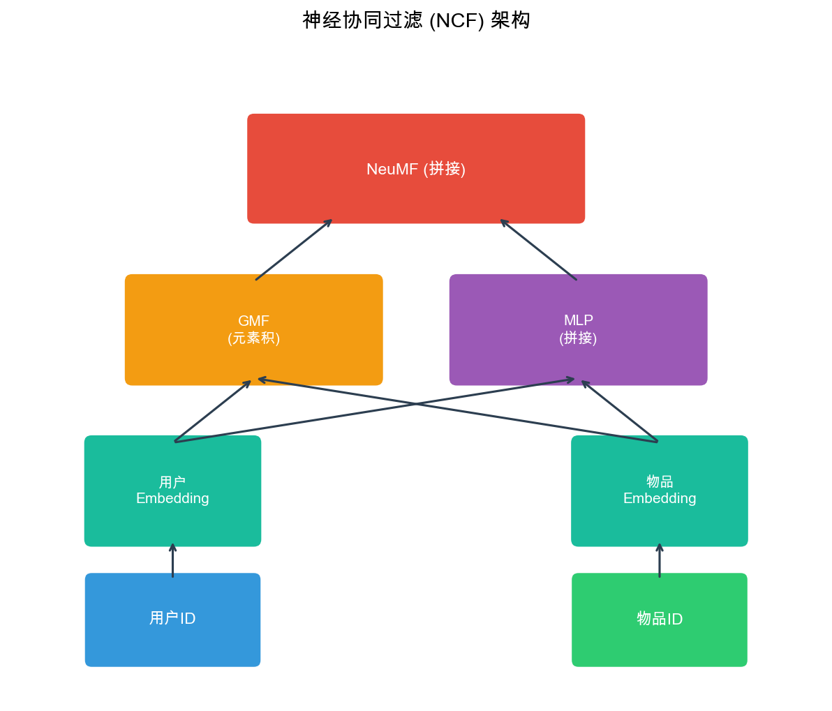
NCF Model Architecture
The NCF model contains three components:
1. GMF (Generalized Matrix Factorization): - User Embedding:\(\mathbf{p}_u \in \mathbb{R}^d\) - Item Embedding:\(\mathbf{q}_i \in \mathbb{R}^d\) - Element-wise product:\(\mathbf{p}_u \odot \mathbf{q}_i\)(element-wise multiplication) - Output:\(\hat{y}_{ui}^{GMF} = \mathbf{h}^T (\mathbf{p}_u \odot \mathbf{q}_i)\), where\(\mathbf{h}\)is a learnable weight vector
2. MLP (Multi-Layer Perceptron): - Concatenate user and item Embeddings:\([\mathbf{p}_u; \mathbf{q}_i]\) - Pass through multi-layer fully connected network:\(\mathbf{z}_1 = \text{ReLU}(\mathbf{W}_1 [\mathbf{p}_u; \mathbf{q}_i] + \mathbf{b}_1)\) -\(\mathbf{z}_2 = \text{ReLU}(\mathbf{W}_2 \mathbf{z}_1 + \mathbf{b}_2)\) - ... - Output:\(\hat{y}_{ui}^{MLP} = \mathbf{h}^T \mathbf{z}_L\) 3. NeuMF (Neural Matrix Factorization): - Fuse GMF and MLP:\(\hat{y}_{ui} = \sigma(\hat{y}_{ui}^{GMF} + \hat{y}_{ui}^{MLP})\) - Where\(\sigma\)is the Sigmoid activation function (for binary classification tasks)
Mathematical Formulation of NCF
The complete NCF model can be expressed as:\[\hat{y}_{ui} = \sigma(\mathbf{h}^T (\mathbf{p}_u \odot \mathbf{q}_i) + \mathbf{h}_{MLP}^T \mathbf{z}_L)\]Where: -\(\mathbf{p}_u, \mathbf{q}_i\): User and item Embedding vectors -\(\odot\): Element-wise product (Hadamard product) -\(\mathbf{z}_L\): Output of the last layer of MLP -\(\mathbf{h}, \mathbf{h}_{MLP}\): Weight vectors of the output layer -\(\sigma\): Sigmoid function
Loss Function of NCF
For implicit feedback (click/no-click), NCF uses binary cross-entropy loss:\[\mathcal{L} = -\sum_{(u,i) \in \mathcal{D }} y_{ui} \log \hat{y}_{ui} + (1-y_{ui}) \log(1-\hat{y}_{ui})\]Where\(y_{ui} \in \{0,1\}\)indicates whether user\(u\)interacted with item\(i\).
For explicit feedback (ratings), mean squared error can be used:\[\mathcal{L} = \sum_{(u,i) \in \mathcal{D }} (r_{ui} - \hat{r}_{ui})^2\]
Complete NCF Implementation
1 | import torch |
NCF Training Tips
1. Negative Sampling: - For implicit feedback, negative samples (no-click) far outnumber positive samples (click) - Need negative sampling to balance positive/negative sample ratio - Common ratio: positive:negative = 1:1 to 1:4
2. Learning Rate Scheduling: - Initial learning rate: 0.001-0.01 - Use learning rate decay (e.g., halve every 10 epochs) - Or use adaptive optimizers (Adam, AdamW)
3. Regularization: - L2 regularization: Prevent overfitting - Dropout: Use in MLP layers, dropout rate 0.2-0.5 - Early Stopping: Monitor validation set performance
4. Pre-training: - Pre-train GMF and MLP separately first - Then jointly train with NeuMF - Can accelerate convergence and improve performance
AutoEncoder Recommendations: CDAE and VAE
Basic Idea of AutoEncoder
AutoEncoder is an unsupervised learning model that attempts to learn low-dimensional representations (encoding) of data, then reconstructs the original data (decoding) from the low-dimensional representation.
In recommendation systems, AutoEncoders can be used to: 1. Dimensionality Reduction: Compress high-dimensional user-item interaction matrices to low-dimensional space 2. Denoising: Recover complete user preferences from sparse, noisy interaction data 3. Generation: Generate items users might be interested in
CDAE: Collaborative Denoising Auto-Encoder
CDAE (Collaborative Denoising Auto-Encoder), proposed in 2015, takes user interaction history as input and reconstructs complete user preferences through a denoising autoencoder.
Model Architecture: - Input Layer: User interaction vector\(\mathbf{x}_u \in \{0,1} ^n\)(\(n\)is the number of items) - Encoder Layer:\(\mathbf{h}_u = \sigma(\mathbf{W} \mathbf{x}_u + \mathbf{V} \mathbf{p}_u + \mathbf{b})\), where\(\mathbf{p}_u\)is the user Embedding - Decoder Layer:\(\hat{\mathbf{x }}_u = \sigma(\mathbf{W}' \mathbf{h}_u + \mathbf{b}')\) - Loss Function: Reconstruction error\(\mathcal{L} = \sum_{u} \|\mathbf{x}_u - \hat{\mathbf{x }}_u\|^2\) Denoising Mechanism: - Randomly zero out part of the input during training (dropout) - Forces the model to learn to recover complete information from partial information - Improves model robustness
Complete CDAE Implementation
1 | import torch |
VAE: Variational Auto-Encoder
VAE (Variational Auto-Encoder), proposed in 2013, is a generative model that probabilizes AutoEncoders, learning latent distributions of data to generate new samples.
In recommendation systems, VAE can be used to: 1. Generate Recommendations: Sample from user latent distributions to generate items of interest 2. Uncertainty Modeling: Not only predict ratings but also predict uncertainty 3. Diverse Recommendations: Increase recommendation diversity through sampling
Mathematical Principles of VAE: - Encoder: Learns posterior distribution\(q_\phi(\mathbf{z}|\mathbf{x})\), where\(\mathbf{z}\)is the latent variable - Decoder: Learns generative distribution\(p_\theta(\mathbf{x}|\mathbf{z})\) - Loss Function: ELBO (Evidence Lower BOund)\[\mathcal{L} = \mathbb{E}_{q_\phi(\mathbf{z}|\mathbf{x})}[\log p_\theta(\mathbf{x}|\mathbf{z})] - \text{KL}(q_\phi(\mathbf{z}|\mathbf{x}) \| p(\mathbf{z}))\]
VAE Recommendation Model (Mult-VAE)
Mult-VAE, proposed in 2018, is a VAE recommendation model that assumes user interaction vectors follow a multinomial distribution.
Model Architecture: - Encoder:\(\mathbf{z}_u \sim \mathcal{N}(\boldsymbol{\mu}_u, \text{diag}(\boldsymbol{\sigma}_u^2))\) -\(\boldsymbol{\mu}_u = \mathbf{W}_\mu \mathbf{h}_u + \mathbf{b}_\mu\) -\(\log \boldsymbol{\sigma}_u^2 = \mathbf{W}_\sigma \mathbf{h}_u + \mathbf{b}_\sigma\) - Where\(\mathbf{h}_u\)is the encoding of user interaction vector - Sampling:\(\mathbf{z}_u = \boldsymbol{\mu}_u + \boldsymbol{\sigma}_u \odot \boldsymbol{\epsilon}\), where\(\boldsymbol{\epsilon} \sim \mathcal{N}(0, \mathbf{I})\) - Decoder:\(\hat{\mathbf{x }}_u = \text{softmax}(\mathbf{W}_d \mathbf{z}_u + \mathbf{b}_d)\)
Complete Mult-VAE Implementation
1 | import torch |
CDAE vs VAE Comparison
| Feature | CDAE | VAE |
|---|---|---|
| Model Type | Deterministic autoencoder | Probabilistic generative model |
| Latent Variable | Fixed vector | Probability distribution |
| Generation Capability | Weak (can only reconstruct) | Strong (can sample and generate) |
| Uncertainty | Cannot model | Can model |
| Training Difficulty | Simple | More complex (requires KL divergence) |
| Recommendation Diversity | Lower | Higher (through sampling) |
| Applicable Scenarios | Dense interaction data | Sparse interaction data |
Wide & Deep Model
Background of Wide & Deep
In 2016, Google proposed the Wide & Deep model in Google Play's recommendation system. The core idea of this model is: combining memorization and generalization.
- Memorization (Wide part): Learns direct associations between features, such as "users who installed Pandora also installed YouTube"
- Generalization (Deep part): Learns Embedding representations of features, capturing latent associations between sparse features
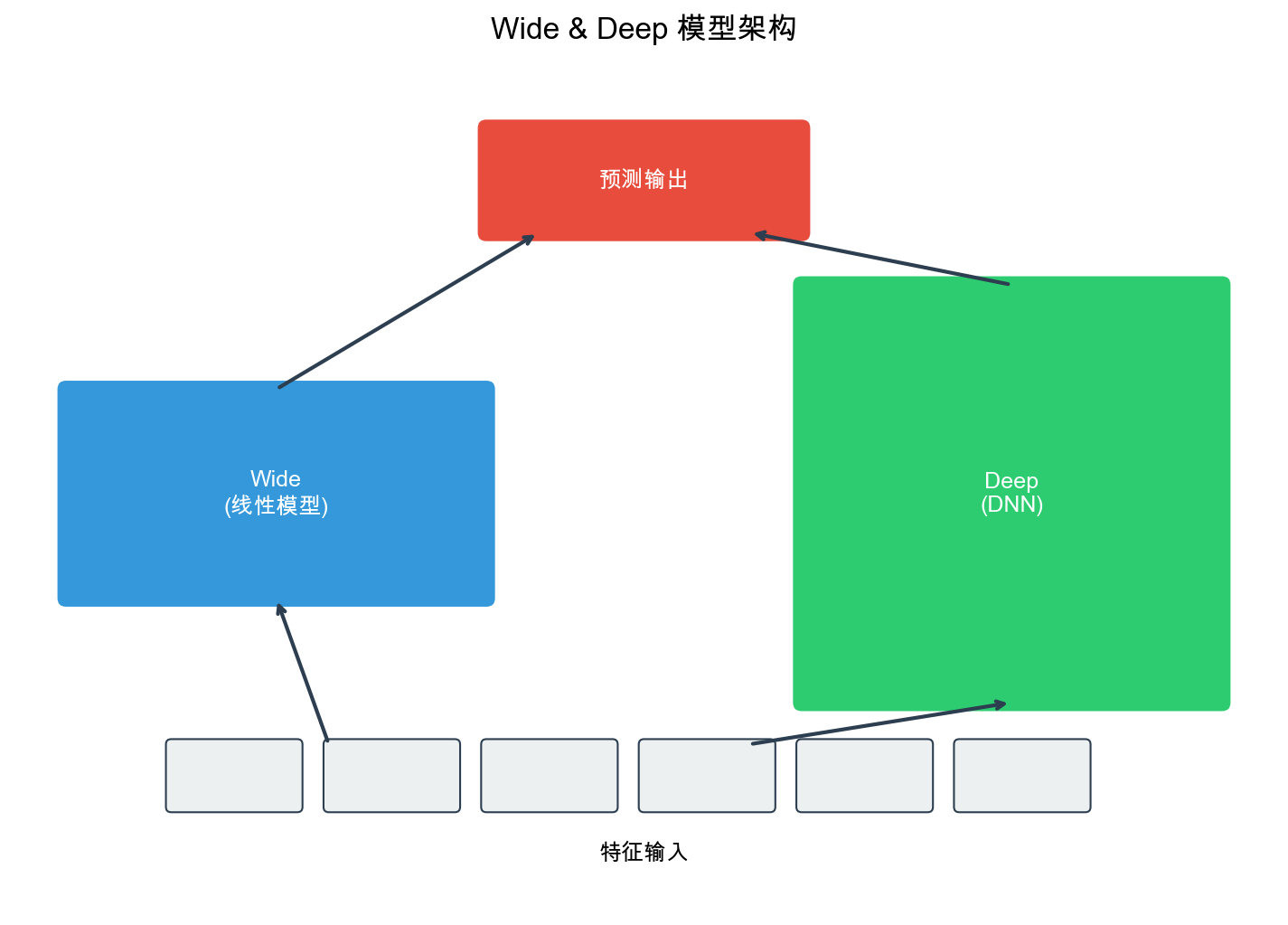
Wide & Deep Model Architecture
The Wide & Deep model contains two components:
1. Wide Part (Linear Model): - Input: Raw features and cross features (e.g., "user age × item category") - Output:\(\hat{y}_{wide} = \mathbf{w}^T \mathbf{x} + b\) - Role: Memorize feature combinations in historical data
2. Deep Part (Deep Neural Network): - Input: Embedding vectors of sparse features - Structure: Multi-layer fully connected network - Output:\(\hat{y}_{deep} = \text{MLP}(\text{Embedding}(\mathbf{x}))\) - Role: Generalize to unseen feature combinations
3. Fusion: - Final output:\(\hat{y} = \sigma(\hat{y}_{wide} + \hat{y}_{deep})\) - Where\(\sigma\)is the Sigmoid function (for CTR prediction)
Mathematical Formulation of Wide & Deep
The complete Wide & Deep model can be expressed as:\[\hat{y} = \sigma(\mathbf{w}_{wide}^T [\mathbf{x}, \phi(\mathbf{x})] + \mathbf{w}_{deep}^T \mathbf{a}^{(L)} + b)\]Where: -\(\mathbf{x}\): Raw features -\(\phi(\mathbf{x})\): Cross features (e.g.,\(\phi(\mathbf{x}) = [x_i \cdot x_j]\)) -\(\mathbf{a}^{(L)}\): Output of the last layer of the Deep part -\(\mathbf{w}_{wide}, \mathbf{w}_{deep}, b\): Learnable parameters
Computation process of the Deep part: -\(\mathbf{a}^{(0)} = \text{Embedding}(\mathbf{x})\) -\(\mathbf{a}^{(l)} = \text{ReLU}(\mathbf{W}^{(l)} \mathbf{a}^{(l-1)} + \mathbf{b}^{(l)})\),\(l=1,2,\dots,L\) - Where\(L\)is the number of layers
Complete Wide & Deep Implementation
1 | import torch |
Optimized Versions of Wide & Deep
In practical applications, Wide & Deep has several optimized versions:
1. DeepFM: - Replaces Wide part with FM - Automatically learns second-order feature interactions - Avoids manual design of cross features
2. xDeepFM: - Introduces CIN (Compressed Interaction Network) - Explicitly models high-order feature interactions - Stronger interaction modeling capability than DeepFM
3. DCN (Deep & Cross Network): - Replaces Wide part with Cross Network - Automatically learns feature interactions of arbitrary order - High computational efficiency
Feature Engineering
Feature Types
Features in recommendation systems can be divided into the following categories:
1. User Features: - User ID, age, gender, city, occupation - User historical behavior statistics (click rate, purchase rate, average rating) - User profile tags (interest tags, consumption ability)
2. Item Features: - Item ID, category, brand, price - Item statistical features (click rate, purchase rate, average rating) - Item content features (text description, images)
3. Context Features: - Time features (hour, day of week, month, whether holiday) - Device features (device type, operating system, APP version) - Location features (GPS coordinates, city, business district)
4. Interaction Features: - User-item interaction history (last N clicks, purchases) - User-category interaction statistics (click counts for each category) - Item-user interaction statistics (user profiles who clicked the item)
5. Cross Features: - User features × item features (e.g., "user age × item category") - Time features × item features (e.g., "time period × item category") - High-order cross features (e.g., "user age × item category × time period")
Feature Encoding
1. Numerical Features: - Standardization:\(x' = \frac{x - \mu}{\sigma}\) - Normalization:\(x' = \frac{x - x_{min }}{x_{max} - x_{min }}\) - Binning: Discretize continuous values, e.g., age divided into "0-18, 19-30, 31-50, 50+"
2. Categorical Features: - One-hot Encoding: One dimension per category - Embedding Encoding: Map to low-dimensional dense vectors (commonly used in deep learning) - Hash Encoding: Use hash function to map categories to fixed dimensions
3. Sequential Features: - Padding: Pad sequences of different lengths to the same length - Pooling: Average pooling, max pooling, attention pooling - RNN/Transformer: Process with sequence models
Feature Selection
Not all features are useful; feature selection is needed:
1. Statistical Methods: - Mutual Information: Measures correlation between features and target - Chi-square Test: Tests independence between features and target - Correlation Coefficient: Computes linear correlation between features and target
2. Model Methods: - L1 Regularization: Automatically sets weights of unimportant features to zero - Feature Importance: Feature importance based on tree models (e.g., XGBoost) - Permutation Importance: Shuffle feature values, observe model performance degradation
3. Business Methods: - A/B Testing: Deploy features, observe metric changes - Feature Analysis: Analyze feature distribution, missing rate, coverage
Feature Engineering Code Example
1 | import numpy as np |
Training Techniques
Data Preparation
1. Negative Sampling: - For implicit feedback, negative samples far outnumber positive samples - Need negative sampling to balance positive/negative sample ratio - Common strategies: random negative sampling, popular negative sampling, hard negative sampling
1 | def negative_sampling(user_items, num_negatives=4): |
2. Data Augmentation: - Time Window Sliding: Build training sets with different time windows - Data Mixing: Mix data from different sources - Noise Injection: Add noise during training to improve robustness
3. Data Splitting: - Time-based Split: Split training and test sets chronologically (more realistic) - Random Split: Random split (may cause data leakage) - User-based Split: Split by users (avoid users appearing in both training and test sets)
Model Training
1. Optimizer Selection: - Adam/AdamW: Adaptive learning rate, suitable for most scenarios - SGD: Requires manual learning rate tuning, but may converge to better solutions - Adagrad: Suitable for sparse gradients
1 | import torch.optim as optim |
2. Learning Rate Scheduling: - StepLR: Decay every N epochs - ExponentialLR: Exponential decay - CosineAnnealingLR: Cosine annealing - ReduceLROnPlateau: Automatically adjust based on validation performance
1 | # StepLR: halve learning rate every 10 epochs |
3. Regularization: - L2 Regularization: Implemented through weight_decay - Dropout: Randomly zero out some neurons - Batch Normalization: Normalize activation values - Early Stopping: Stop early when validation performance doesn't improve
1 | # Dropout |
Training Loop Example
1 | def train_model(model, train_loader, val_loader, num_epochs=50): |
Evaluation Metrics
1. Classification Tasks (CTR Prediction): - AUC: Area under ROC curve, measures ranking capability - LogLoss: Logarithmic loss, measures accuracy of predicted probabilities - Precision@K: Proportion of positive samples in Top-K recommendations - Recall@K: Coverage of positive samples by Top-K recommendations
2. Regression Tasks (Rating Prediction): - RMSE: Root mean squared error - MAE: Mean absolute error - NDCG: Normalized Discounted Cumulative Gain (ranking metric)
1 | from sklearn.metrics import roc_auc_score, log_loss, precision_recall_fscore_support |
Q&A: Common Questions
Q1: How to Choose Embedding Dimensions?
A: The choice of Embedding dimension\(d\)requires balancing model capacity and computational cost:
- Small-scale data (<100K users/items):\(d = 8-16\)is sufficient
- Medium-scale data (100K-1M):\(d = 32-64\)is common
- Large-scale data (>1M):\(d = 64-128\), even 256
Rule of thumb: 1. Start with\(d=32\), gradually increase to 64, 128 2. Observe validation performance; if improvement <1%, stop increasing 3. Consider computational resources: doubling\(d\)doubles the number of parameters
Q2: Why Does NCF Perform Better Than Matrix Factorization?
A: NCF's advantages mainly lie in:
- Nonlinear Modeling: Matrix factorization can only capture linear relationships (inner products), while NCF can capture nonlinear relationships through MLP
- Feature Fusion: NCF's GMF and MLP parts complement each other; GMF captures simple interactions, MLP captures complex interactions
- End-to-End Training: The entire model can be jointly optimized, while matrix factorization typically requires alternating optimization
However, NCF also has disadvantages: - Higher computational complexity (requires forward propagation) - Poor interpretability (black-box model) - Requires more data to train well
Q3: What's the Difference Between CDAE and VAE?
A: Main differences:
- Model Type:
- CDAE: Deterministic autoencoder, latent variable is a fixed vector
- VAE: Probabilistic generative model, latent variable is a probability distribution
- Generation Capability:
- CDAE: Can only reconstruct input, cannot generate new samples
- VAE: Can sample from latent distribution to generate new samples
- Uncertainty:
- CDAE: Cannot model uncertainty
- VAE: Can model uncertainty through variance of latent distribution
- Training:
- CDAE: Simple training, only needs reconstruction loss
- VAE: Requires KL divergence term, more complex training
- Recommendation Diversity:
- CDAE: Recommendation results are relatively fixed
- VAE: Can increase diversity through sampling
Q4: What Are the Respective Roles of Wide and Deep Parts in Wide & Deep?
A:
Wide Part (Memorization): - Learns direct associations between features - Example: "Users who installed Pandora also installed YouTube" - Suitable for handling sparse, high-dimensional cross features - Can quickly memorize patterns in historical data
Deep Part (Generalization): - Learns Embedding representations of features - Captures latent associations between sparse features - Can generalize to unseen feature combinations - Suitable for handling dense Embedding features
Why Combine Both: - Only Wide: Cannot generalize, can only memorize historical data - Only Deep: May over-generalize, ignoring important direct associations - Wide + Deep: Both memorize and generalize, achieving optimal results
Q5: How to Handle Cold Start Problems?
A: Cold start is a classic problem in recommendation systems, with the following solutions:
1. New User Cold Start: - Popular Recommendations: Recommend popular items - Content-based Recommendations: Recommend based on user registration information (age, gender, etc.) - Transfer Learning: Transfer preferences from similar users - Multi-armed Bandit: Exploration-exploitation balance
2. New Item Cold Start: - Content Features: Recommend to similar users based on item attributes (category, tags) - Embedding Pre-training: Pre-train Embeddings using item content features - Collaborative Filtering: Based on interaction data of similar items
3. System Cold Start: - External Data: Leverage data from other platforms - Expert Rules: Manually designed recommendation rules - A/B Testing: Rapid iterative optimization
Q6: How to Choose Negative Sampling Strategies?
A: Negative sampling strategies affect model performance:
1. Random Negative Sampling: - Simplest, randomly sample from all non-interacted items - Suitable for most scenarios - May sample items that "users aren't interested in but don't dislike"
2. Popular Negative Sampling: - Sample negative samples from popular items - Assumes users not clicking popular items means they don't like them - May introduce popularity bias
3. Hard Negative Sampling: - Sample negative samples with high model prediction scores - Let the model learn to distinguish "easily confused" positive and negative samples - Improves model performance but requires dynamic sampling (model changes during training)
4. Mixed Strategy: - 50% random + 50% popular - Or adjust according to training phase: random early, hard negative sampling later
Q7: How to Prevent Overfitting?
A: Methods to prevent overfitting:
1. Regularization: - L2 Regularization: Implemented through weight_decay, typically 1e-5 to 1e-3 - Dropout: Randomly zero out some neurons, dropout rate 0.2-0.5 - Batch Normalization: Normalize activation values, stabilize training
2. Data Augmentation: - Negative Sampling: Increase number of negative samples - Noise Injection: Add noise during training - Data Mixing: Mix data from different sources
3. Model Complexity Control: - Reduce Layers: Start with deep networks, gradually reduce - Reduce Embedding Dimensions: Lower model capacity - Early Stopping: Stop training when validation performance doesn't improve
4. Cross Validation: - Use K-fold cross validation to evaluate models - Avoid randomness of single split
Q8: How to Accelerate Model Training?
A: Methods to accelerate training:
1. Hardware Acceleration: - GPU: Use CUDA acceleration, 10-100x speedup - Multi-GPU: Data parallelism or model parallelism - TPU: Google's specialized chip, suitable for large-scale training
2. Data Optimization: - Data Preprocessing: Preprocess features in advance, avoid computation during training - Data Loading: Use multi-process DataLoader (num_workers>0) - Batch Size: Increase batch size to improve GPU utilization
3. Model Optimization: - Mixed Precision Training: Use FP16, 2x speedup - Gradient Accumulation: Simulate large batch training - Model Pruning: Reduce model parameters
4. Algorithm Optimization: - Learning Rate Scheduling: Use warmup to accelerate convergence - Optimizer Selection: Adam usually converges faster than SGD - Asynchronous Training: Multi-machine multi-GPU asynchronous updates
Q9: How to Evaluate Recommendation System Effectiveness?
A: Recommendation system evaluation requires multi-dimensional metrics:
1. Offline Metrics: - Accuracy Metrics: AUC, LogLoss, RMSE, MAE - Ranking Metrics: NDCG, MRR, MAP - Coverage Metrics: Coverage (diversity of recommended items) - Diversity Metrics: Intra-list Diversity (differences between items in recommendation list)
2. Online Metrics: - CTR: Click-through rate - CVR: Conversion rate (purchase/download) - GMV: Gross merchandise value - User Retention Rate: Proportion of returning users
3. Business Metrics: - User Satisfaction: Ratings, feedback - Long-tail Item Recommendations: Whether unpopular items are recommended - Real-time Performance: Recommendation response time
4. A/B Testing: - Compare effects of old and new models - Requires sufficient sample size (typically >1000 users) - Focus on statistical significance
Q10: Can Embeddings Be Visualized?
A: Yes, common visualization methods:
1. t-SNE: - Reduce high-dimensional Embeddings to 2D - Can observe whether similar items cluster - Suitable for exploratory analysis
2. PCA: - Linear dimensionality reduction, fast computation - Preserves main variance - Suitable for preliminary analysis
3. UMAP: - Faster than t-SNE, similar effects - Preserves local and global structure - Suitable for large-scale data
4. Visualization Tools: - TensorBoard: TensorFlow's visualization tool - Weights & Biases: Online visualization platform - Plotly: Interactive visualization
Visualization can help: - Understand what the model has learned - Discover anomalies (e.g., some item Embeddings are abnormal) - Explain recommendation results (why this item is recommended)
Q11: How to Handle New Categories in Categorical Features?
A: New categories (OOV, Out-of-Vocabulary) are common problems:
1. Default Embedding: - Assign a special Embedding vector to new categories - Can randomly initialize or use zero vector - Will be updated during training
2. Hash Trick: - Use hash function to map new
categories to known categories - Example:
hash(new_category) % num_categories - May have hash
collisions but can handle arbitrary new categories
3. Content Features: - If new categories have content features (e.g., text description), can initialize Embeddings with content features - Example: Encode category names with Word2Vec
4. Transfer Learning: - Transfer Embeddings from similar categories - Example: New movie categories can initialize Embeddings with similar categories
Q12: How to Combine Deep Learning Recommendation Models with Traditional Methods?
A: Can combine in various ways:
1. Model Fusion: - Weighted Average: Weighted average of predictions from multiple models - Stacking: Use meta-model to learn how to combine multiple models - Blending: Different models responsible for different scenarios
2. Feature Fusion: - Outputs of traditional methods as input features for deep learning models - Example: Prediction scores from matrix factorization as features
3. Two-stage Recommendation: - Recall Stage: Use traditional methods (e.g., Item-CF) to quickly recall candidate sets - Ranking Stage: Use deep learning models for fine-grained ranking
4. Ensemble Learning: - Train multiple models with different structures - Vote or average to get final results - Usually performs better than single models
Summary
Deep learning has brought revolutionary changes to recommendation systems. From automatic feature learning through Embeddings, to nonlinear modeling with NCF, from denoising reconstruction with AutoEncoders, to combining memorization and generalization with Wide & Deep, deep learning models have demonstrated powerful capabilities across all recommendation scenarios.
However, deep learning is not a silver bullet. It requires large amounts of data, computational resources, and tuning experience. In practical applications, we need to: 1. Understand Business Scenarios: Choose appropriate model architectures 2. Do Feature Engineering Well: Feature quality determines the model's upper limit 3. Carefully Design Training Pipelines: Data preparation, negative sampling, regularization, evaluation metrics 4. Continuously Iterate and Optimize: A/B testing, online monitoring, rapid iteration
Recommendation systems are complex engineering systems, and deep learning is just one component. Only by combining algorithms, engineering, and business can we build truly effective recommendation systems.
Future directions for recommendation systems include: - Sequential Recommendations: Use Transformer to model user behavior sequences - Reinforcement Learning: Dynamically adjust recommendation strategies - Multimodal Recommendations: Fuse text, images, video, and other modalities - Explainable Recommendations: Help users understand why items are recommended - Fair Recommendations: Avoid recommendation bias, protect user privacy
I hope this article helps you build a complete knowledge framework for deep learning recommendation systems. If you have any questions, feel free to discuss them in the comments.
- Post title:Recommendation Systems (3): Deep Learning Foundation Models
- Post author:Chen Kai
- Create time:2026-02-03 23:11:11
- Post link:https://www.chenk.top/recommendation-systems-3-deep-learning-basics/
- Copyright Notice:All articles in this blog are licensed under BY-NC-SA unless stating additionally.