Recommendation Systems (15): Real-Time Recommendation and Online Learning

permalink: "en/recommendation-systems-15-real-time-online/" date: 2024-07-11 10:15:00 tags: - Recommendation Systems - Real-Time - Online Learning categories: Recommendation Systems mathjax: true--- In the era of instant gratification, recommendation systems face an unprecedented challenge: users expect personalized suggestions that adapt to their current interests within milliseconds. Traditional batch-based approaches, which retrain models every few hours or days, simply cannot keep pace with rapidly changing user preferences, trending content, or contextual shifts. This article explores real-time recommendation architectures and online learning algorithms that enable systems to learn and adapt continuously from streaming data, making decisions in real-time while balancing exploration and exploitation.

Introduction: The Need for Real-Time Adaptation

Consider a user browsing an e-commerce platform. At 2 PM, they're searching for hiking gear. By 3 PM, they've shifted to looking at books. A traditional recommendation system trained on yesterday's data would still be suggesting hiking boots, completely missing the user's current intent. Real-time recommendation systems solve this by continuously updating their understanding of user preferences as new interactions arrive, often processing thousands of events per second while maintaining sub-100ms latency for serving recommendations.

The core challenge lies in the exploration-exploitation dilemma: should the system exploit what it knows works well, or explore new options to discover potentially better recommendations? Online learning algorithms, particularly multi-armed bandits and their contextual extensions, provide principled solutions to this problem, enabling systems to learn optimal strategies while serving users.

Real-Time Architecture Fundamentals

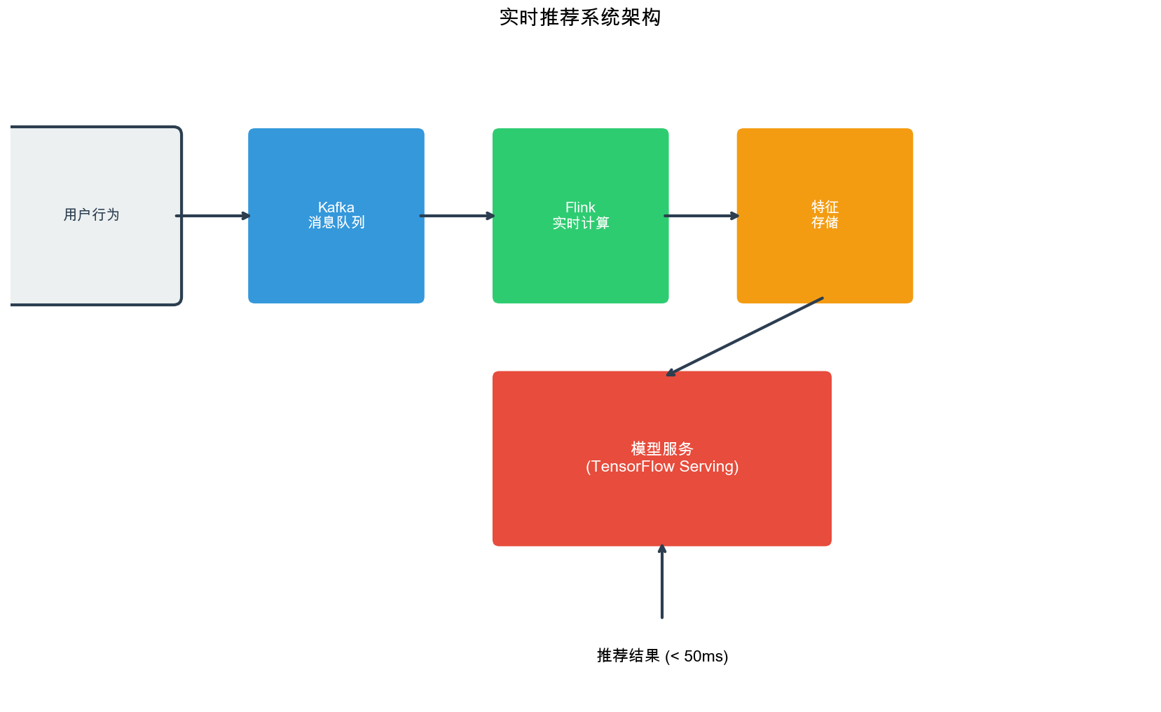
System Components

A real-time recommendation system typically consists of several interconnected components:

1. Event Ingestion Layer: Captures user interactions (clicks, views, purchases) as they occur
2. Stream Processing Engine: Processes events in real-time, updating feature stores and model parameters
3. Feature Store: Maintains up-to-date user and item features accessible with low latency
4. Model Serving Layer: Serves predictions using the latest model state
5. Feedback Loop: Ensures model updates influence future recommendations

Latency Requirements

Different components have different latency budgets:

• Event ingestion: < 10ms (must not block user interactions)
• Feature computation: < 50ms (for real-time features)
• Model inference: < 50ms (for ranking/scoring)
• Total end-to-end: < 100ms (for user-facing recommendations)

These constraints necessitate careful architecture design, often involving in-memory stores, pre-computed features, and efficient model formats.

Streaming Frameworks: Apache Kafka and Apache Flink

Apache Kafka: Event Streaming Platform

Kafka serves as the backbone for event ingestion and distribution. It provides:

• High throughput: Millions of messages per second
• Durability: Persistent storage with configurable retention
• Scalability: Horizontal scaling through partitioning
• Consumer groups: Enable parallel processing while maintaining ordering guarantees

Kafka Setup for Recommendation Events

from kafka import KafkaProducer, KafkaConsumer
import json
from datetime import datetime

class RecommendationEventProducer:
    """Produces recommendation events to Kafka."""
    
    def __init__(self, bootstrap_servers=['localhost:9092']):
        self.producer = KafkaProducer(
            bootstrap_servers=bootstrap_servers,
            value_serializer=lambda v: json.dumps(v).encode('utf-8'),
            key_serializer=lambda k: k.encode('utf-8') if k else None
        )
    
    def send_interaction_event(self, user_id, item_id, event_type, 
                              timestamp=None, metadata=None):
        """Send a user interaction event."""
        event = {
            'user_id': user_id,
            'item_id': item_id,
            'event_type': event_type,  # 'click', 'view', 'purchase', 'skip'
            'timestamp': timestamp or datetime.utcnow().isoformat(),
            'metadata': metadata or {}
        }
        
        # Partition by user_id for ordering guarantees per user
        future = self.producer.send(
            'user-interactions',
            key=str(user_id),
            value=event
        )
        return future
    
    def send_impression_event(self, user_id, item_ids, context=None):
        """Send an impression event (items shown to user)."""
        event = {
            'user_id': user_id,
            'item_ids': item_ids,
            'context': context or {},
            'timestamp': datetime.utcnow().isoformat()
        }
        self.producer.send('impressions', key=str(user_id), value=event)

# Usage example
producer = RecommendationEventProducer()
producer.send_interaction_event(
    user_id='user_123',
    item_id='item_456',
    event_type='click',
    metadata={'position': 3, 'session_id': 'sess_789'}
)

Kafka Consumer for Real-Time Processing

from kafka import KafkaConsumer
import json
from collections import defaultdict

class RealTimeFeatureUpdater:
    """Consumes events and updates features in real-time."""
    
    def __init__(self, bootstrap_servers=['localhost:9092']):
        self.consumer = KafkaConsumer(
            'user-interactions',
            bootstrap_servers=bootstrap_servers,
            value_deserializer=lambda m: json.loads(m.decode('utf-8')),
            group_id='feature-updater-group',
            auto_offset_reset='latest',
            enable_auto_commit=True
        )
        self.user_features = defaultdict(dict)
        self.item_features = defaultdict(dict)
    
    def process_event(self, event):
        """Process a single event and update features."""
        user_id = event['user_id']
        item_id = event['item_id']
        event_type = event['event_type']
        
        # Update user activity features
        if 'last_activity' not in self.user_features[user_id]:
            self.user_features[user_id]['last_activity'] = event['timestamp']
        
        # Update click-through rate features
        if 'clicks' not in self.user_features[user_id]:
            self.user_features[user_id]['clicks'] = 0
        if 'views' not in self.user_features[user_id]:
            self.user_features[user_id]['views'] = 0
        
        if event_type == 'click':
            self.user_features[user_id]['clicks'] += 1
        elif event_type == 'view':
            self.user_features[user_id]['views'] += 1
        
        # Calculate CTR
        if self.user_features[user_id]['views'] > 0:
            self.user_features[user_id]['ctr'] = (
                self.user_features[user_id]['clicks'] / 
                self.user_features[user_id]['views']
            )
        
        # Update item popularity
        if event_type == 'click':
            if 'clicks' not in self.item_features[item_id]:
                self.item_features[item_id]['clicks'] = 0
            self.item_features[item_id]['clicks'] += 1
    
    def run(self):
        """Main processing loop."""
        for message in self.consumer:
            try:
                event = message.value
                self.process_event(event)
            except Exception as e:
                print(f"Error processing event: {e}")

Apache Flink: Stream Processing Engine

Flink provides powerful stream processing capabilities with:

• Low latency: Sub-second processing
• Exactly-once semantics: Guaranteed processing without duplicates
• Stateful processing: Maintains state across events
• Event time handling: Handles out-of-order events correctly

Flink Job for Real-Time Recommendations

from pyflink.datastream import StreamExecutionEnvironment
from pyflink.table import StreamTableEnvironment
from pyflink.datastream.functions import MapFunction, KeyedProcessFunction
from pyflink.common.typeinfo import Types
from pyflink.common.time import Time
import json

class InteractionEventParser(MapFunction):
    """Parse JSON events from Kafka."""
    
    def map(self, value):
        event = json.loads(value)
        return (
            event['user_id'],
            event['item_id'],
            event['event_type'],
            event['timestamp']
        )

class RealTimeCTRCalculator(KeyedProcessFunction):
    """Calculate CTR in real-time using Flink state."""
    
    def __init__(self):
        self.clicks_state = None
        self.views_state = None
    
    def open(self, runtime_context):
        # Initialize state descriptors
        from pyflink.datastream.state import ValueStateDescriptor
        
        clicks_desc = ValueStateDescriptor("clicks", Types.LONG())
        views_desc = ValueStateDescriptor("views", Types.LONG())
        
        self.clicks_state = runtime_context.get_state(clicks_desc)
        self.views_state = runtime_context.get_state(views_desc)
    
    def process_element(self, value, ctx, out):
        user_id, item_id, event_type, timestamp = value
        
        # Update state
        clicks = self.clicks_state.value() or 0
        views = self.views_state.value() or 0
        
        if event_type == 'click':
            clicks += 1
            self.clicks_state.update(clicks)
        elif event_type == 'view':
            views += 1
            self.views_state.update(views)
        
        # Calculate and emit CTR
        if views > 0:
            ctr = clicks / views
            out.collect((user_id, ctr, clicks, views))

# Flink job setup
env = StreamExecutionEnvironment.get_execution_environment()
env.set_stream_time_characteristic(TimeCharacteristic.EventTime)

# Create table environment for SQL API
table_env = StreamTableEnvironment.create(env)

# Define Kafka source
table_env.execute_sql("""
    CREATE TABLE user_interactions (
        user_id STRING,
        item_id STRING,
        event_type STRING,
        event_time TIMESTAMP(3),
        WATERMARK FOR event_time AS event_time - INTERVAL '5' SECOND
    ) WITH (
        'connector' = 'kafka',
        'topic' = 'user-interactions',
        'properties.bootstrap.servers' = 'localhost:9092',
        'format' = 'json'
    )
""")

# Process with Flink SQL
result = table_env.execute_sql("""
    SELECT 
        user_id,
        COUNT(CASE WHEN event_type = 'click' THEN 1 END) as clicks,
        COUNT(CASE WHEN event_type = 'view' THEN 1 END) as views,
        COUNT(CASE WHEN event_type = 'click' THEN 1 END) * 1.0 / 
        COUNT(CASE WHEN event_type = 'view' THEN 1 END) as ctr
    FROM user_interactions
    GROUP BY user_id, TUMBLE(event_time, INTERVAL '1' MINUTE)
""")

Online Learning Basics

Batch vs. Online Learning

Batch learning processes all training data at once: - Requires full dataset before training - Computationally expensive for large datasets - Cannot adapt to new patterns quickly - Suitable for stable environments

Online learning processes data one example (or mini-batch) at a time: - Updates model incrementally - Adapts to distribution shifts - Lower memory footprint - Suitable for dynamic environments

Stochastic Gradient Descent (SGD)

The foundation of online learning, SGD updates model parameters after each example:

\[\theta_{t+1} = \theta_t - \eta_t \nabla_\theta L(f(x_t, \theta_t), y_t)\]where\(\eta_t\)is the learning rate at time\(t\), and\(L\)is the loss function.

Online SGD Implementation

import numpy as np
from typing import List, Tuple

class OnlineSGD:
    """Online Stochastic Gradient Descent for recommendation models."""
    
    def __init__(self, n_features, learning_rate=0.01, 
                 learning_rate_decay=0.95):
        self.theta = np.random.normal(0, 0.01, n_features)
        self.learning_rate = learning_rate
        self.learning_rate_decay = learning_rate_decay
        self.t = 0
    
    def update(self, x: np.ndarray, y: float):
        """Update model with a single example."""
        self.t += 1
        
        # Adaptive learning rate
        eta = self.learning_rate / (1 + self.learning_rate_decay * self.t)
        
        # Prediction
        pred = np.dot(self.theta, x)
        
        # Gradient (for squared loss)
        error = pred - y
        gradient = error * x
        
        # Update parameters
        self.theta -= eta * gradient
        
        return pred, error
    
    def predict(self, x: np.ndarray):
        """Make prediction."""
        return np.dot(self.theta, x)

# Example: Online learning for CTR prediction
model = OnlineSGD(n_features=100)

# Simulate streaming data
for i in range(1000):
    # Generate feature vector (user-item features)
    x = np.random.randn(100)
    # True CTR (simulated)
    y = 0.3 + 0.1 * np.sin(i / 100)
    
    pred, error = model.update(x, y)
    
    if i % 100 == 0:
        print(f"Step {i}: Prediction={pred:.4f}, Error={error:.4f}")

Per-Coordinate Learning Rates

Different features may require different learning rates. AdaGrad adapts learning rates per coordinate:\[g_{t,i} = \nabla_{\theta_i} L(f(x_t, \theta_t), y_t)\] \[G_{t,i} = \sum_{s=1}^t g_{s,i}^2\] \[\theta_{t+1,i} = \theta_{t,i} - \frac{\eta}{\sqrt{G_{t,i} + \epsilon }} g_{t,i}\]

AdaGrad Implementation

class AdaGrad:
    """AdaGrad with per-coordinate adaptive learning rates."""
    
    def __init__(self, n_features, learning_rate=0.01, epsilon=1e-8):
        self.theta = np.zeros(n_features)
        self.learning_rate = learning_rate
        self.epsilon = epsilon
        self.G = np.zeros(n_features)  # Sum of squared gradients
    
    def update(self, x: np.ndarray, y: float):
        """Update with AdaGrad."""
        pred = np.dot(self.theta, x)
        error = pred - y
        gradient = error * x
        
        # Update sum of squared gradients
        self.G += gradient ** 2
        
        # Per-coordinate learning rates
        adaptive_lr = self.learning_rate / (np.sqrt(self.G) + self.epsilon)
        
        # Update parameters
        self.theta -= adaptive_lr * gradient
        
        return pred, error

Multi-Armed Bandits: Exploration vs. Exploitation

The multi-armed bandit problem formalizes the exploration-exploitation trade-off. Imagine a slot machine with multiple arms, each with an unknown reward distribution. The goal is to maximize cumulative reward while learning which arms are best.

Problem Formulation

• Arms:\(K\)actions (e.g.,\(K\)different recommendation strategies)
• Rewards: Each arm\(i\)has expected reward\(\mu_i\)
• Objective: Maximize\(\sum_{t=1}^T r_{a_t}\)where\(a_t\)is the arm chosen at time\(t\)The regret measures performance:\[R_T = T \mu^* - \sum_{t=1}^T \mu_{a_t}\]where\(\mu^* = \max_i \mu_i\)is the optimal arm's expected reward.

Upper Confidence Bound (UCB)

UCB balances exploration and exploitation by choosing arms with high upper confidence bounds:\[a_t = \arg\max_{i=1,\dots,K} \left( \hat{\mu}_i + c \sqrt{\frac{\ln t}{n_i }} \right)\]where: -\(\hat{\mu}_i\)is the empirical mean reward for arm\(i\) -\(n_i\)is the number of times arm\(i\)has been pulled -\(c\)is the exploration parameter (typically\(c = \sqrt{2}\))

UCB Implementation

import math
from collections import defaultdict

class UCB:
    """Upper Confidence Bound algorithm for multi-armed bandits."""
    
    def __init__(self, n_arms, c=math.sqrt(2)):
        self.n_arms = n_arms
        self.c = c
        self.counts = [0] * n_arms
        self.values = [0.0] * n_arms
        self.total_counts = 0
    
    def select_arm(self):
        """Select arm using UCB."""
        for arm in range(self.n_arms):
            if self.counts[arm] == 0:
                return arm  # Explore unplayed arms
        
        ucb_values = []
        for arm in range(self.n_arms):
            confidence = self.c * math.sqrt(
                math.log(self.total_counts) / self.counts[arm]
            )
            ucb_value = self.values[arm] + confidence
            ucb_values.append(ucb_value)
        
        return ucb_values.index(max(ucb_values))
    
    def update(self, arm, reward):
        """Update arm statistics after receiving reward."""
        self.counts[arm] += 1
        self.total_counts += 1
        
        # Update empirical mean
        n = self.counts[arm]
        self.values[arm] = ((n - 1) * self.values[arm] + reward) / n

# Example: UCB for recommendation
bandit = UCB(n_arms=5)  # 5 different recommendation strategies

rewards_by_arm = {
    0: lambda: np.random.binomial(1, 0.1),  # 10% CTR
    1: lambda: np.random.binomial(1, 0.3),  # 30% CTR
    2: lambda: np.random.binomial(1, 0.5),  # 50% CTR (best)
    3: lambda: np.random.binomial(1, 0.2),  # 20% CTR
    4: lambda: np.random.binomial(1, 0.15), # 15% CTR
}

total_reward = 0
for t in range(1000):
    arm = bandit.select_arm()
    reward = rewards_by_arm[arm]()
    bandit.update(arm, reward)
    total_reward += reward
    
    if t % 100 == 0:
        print(f"Step {t}: Selected arm={arm}, Reward={reward}, "
              f"Total reward={total_reward}")

Thompson Sampling

Thompson Sampling is a Bayesian approach that maintains a probability distribution over arm rewards and samples from the posterior to select arms.

For Bernoulli rewards, we use Beta distributions:

• Prior:\(\text{Beta}(\alpha_i, \beta_i)\)for arm\(i\)
• After observing\(s_i\)successes and\(f_i\)failures:\(\text{Beta}(\alpha_i + s_i, \beta_i + f_i)\)
• Select arm by sampling from posteriors:\(a_t = \arg\max_i \theta_i\)where\(\theta_i \sim \text{Beta}(\alpha_i + s_i, \beta_i + f_i)\)

Thompson Sampling Implementation

import numpy as np
from scipy.stats import beta

class ThompsonSampling:
    """Thompson Sampling for Bernoulli bandits."""
    
    def __init__(self, n_arms, alpha=1.0, beta=1.0):
        self.n_arms = n_arms
        self.alpha = np.ones(n_arms) * alpha  # Success counts
        self.beta = np.ones(n_arms) * beta   # Failure counts
    
    def select_arm(self):
        """Select arm by sampling from posterior distributions."""
        samples = []
        for arm in range(self.n_arms):
            # Sample from Beta distribution
            sample = np.random.beta(self.alpha[arm], self.beta[arm])
            samples.append(sample)
        
        return np.argmax(samples)
    
    def update(self, arm, reward):
        """Update Beta distribution parameters."""
        if reward == 1:
            self.alpha[arm] += 1
        else:
            self.beta[arm] += 1
    
    def get_expected_rewards(self):
        """Get expected reward for each arm."""
        return self.alpha / (self.alpha + self.beta)

# Example usage
ts = ThompsonSampling(n_arms=5)

for t in range(1000):
    arm = ts.select_arm()
    # Simulate reward (arm 2 is best with 50% success rate)
    true_probs = [0.1, 0.3, 0.5, 0.2, 0.15]
    reward = np.random.binomial(1, true_probs[arm])
    ts.update(arm, reward)
    
    if t % 200 == 0:
        expected = ts.get_expected_rewards()
        print(f"Step {t}: Expected rewards = {expected}")

Contextual Bandits

Contextual bandits extend multi-armed bandits by incorporating context (features) into decision-making. Instead of learning which arm is best overall, we learn which arm is best given the current context.

Linear Contextual Bandits

In linear contextual bandits, the expected reward is linear in the context:\[E[r_{a_t} | x_t] = x_t^T \theta_{a_t}\]where\(x_t\)is the context vector and\(\theta_{a_t}\)is the parameter vector for arm\(a_t\).

LinUCB: Linear Upper Confidence Bound

LinUCB extends UCB to linear contextual bandits:\[a_t = \arg\max_{a \in A} \left( x_t^T \hat{\theta}_a + \alpha \sqrt{x_t^T A_a^{-1} x_t} \right)\]where: -\(\hat{\theta}_a\)is the estimated parameter for arm\(a\) -\(A_a = D_a^T D_a + I_d\)is the regularized design matrix -\(D_a\)is the matrix of contexts where arm\(a\)was chosen -\(\alpha\)controls exploration

LinUCB Implementation

import numpy as np
from numpy.linalg import inv

class LinUCB:
    """Linear Upper Confidence Bound for contextual bandits."""
    
    def __init__(self, n_arms, n_features, alpha=1.0):
        self.n_arms = n_arms
        self.n_features = n_features
        self.alpha = alpha
        
        # Initialize for each arm
        self.A = [np.eye(n_features)] * n_arms  # Design matrices
        self.b = [np.zeros(n_features)] * n_arms  # Reward vectors
        self.theta = [np.zeros(n_features)] * n_arms  # Parameter estimates
    
    def select_arm(self, context):
        """Select arm given context."""
        context = np.array(context).reshape(-1, 1)
        
        ucb_values = []
        for arm in range(self.n_arms):
            # Compute parameter estimate
            A_inv = inv(self.A[arm])
            self.theta[arm] = A_inv @ self.b[arm]
            
            # Compute UCB
            p = self.theta[arm].T @ context
            uncertainty = self.alpha * np.sqrt(context.T @ A_inv @ context)
            ucb = p + uncertainty
            ucb_values.append(ucb[0, 0])
        
        return np.argmax(ucb_values)
    
    def update(self, arm, context, reward):
        """Update arm parameters after observing reward."""
        context = np.array(context).reshape(-1, 1)
        
        # Update design matrix and reward vector
        self.A[arm] += context @ context.T
        self.b[arm] += reward * context.flatten()
        
        # Update parameter estimate
        A_inv = inv(self.A[arm])
        self.theta[arm] = A_inv @ self.b[arm]

# Example: Contextual bandit for personalized recommendations
linucb = LinUCB(n_arms=3, n_features=5, alpha=1.0)

# Simulate user contexts and rewards
for t in range(500):
    # Generate context (user features)
    context = np.random.randn(5)
    
    # Select arm
    arm = linucb.select_arm(context)
    
    # True reward depends on context and arm
    true_theta = [
        np.array([0.5, 0.3, 0.1, 0.2, 0.4]),  # Arm 0
        np.array([0.2, 0.5, 0.4, 0.3, 0.1]),  # Arm 1
        np.array([0.1, 0.2, 0.5, 0.4, 0.3]),  # Arm 2
    ]
    true_reward = context @ true_theta[arm] + np.random.normal(0, 0.1)
    
    # Update
    linucb.update(arm, context, true_reward)
    
    if t % 100 == 0:
        print(f"Step {t}: Selected arm={arm}, Reward={true_reward:.3f}")

Neural Contextual Bandits

For non-linear relationships, we can use neural networks:

import torch
import torch.nn as nn
import torch.optim as optim

class NeuralContextualBandit(nn.Module):
    """Neural network for contextual bandits."""
    
    def __init__(self, n_features, n_arms, hidden_dim=64):
        super().__init__()
        self.n_arms = n_arms
        
        # Shared feature extractor
        self.feature_extractor = nn.Sequential(
            nn.Linear(n_features, hidden_dim),
            nn.ReLU(),
            nn.Linear(hidden_dim, hidden_dim),
            nn.ReLU()
        )
        
        # Arm-specific heads
        self.arm_heads = nn.ModuleList([
            nn.Linear(hidden_dim, 1) for _ in range(n_arms)
        ])
    
    def forward(self, context):
        """Forward pass."""
        features = self.feature_extractor(context)
        rewards = torch.stack([
            head(features) for head in self.arm_heads
        ], dim=1)
        return rewards.squeeze(-1)
    
    def select_arm(self, context, exploration_bonus=1.0):
        """Select arm with exploration bonus."""
        self.eval()
        with torch.no_grad():
            rewards = self.forward(context)
            # Add exploration bonus (simplified)
            ucb_rewards = rewards + exploration_bonus * torch.randn_like(rewards)
            return torch.argmax(ucb_rewards).item()

# Training loop
model = NeuralContextualBandit(n_features=10, n_arms=5)
optimizer = optim.Adam(model.parameters(), lr=0.001)

contexts = []
arms = []
rewards = []

for t in range(1000):
    # Generate context
    context = torch.randn(1, 10)
    
    # Select arm
    arm = model.select_arm(context)
    
    # Simulate reward
    reward = torch.rand(1).item()
    
    # Store for batch update
    contexts.append(context)
    arms.append(arm)
    rewards.append(reward)
    
    # Update every 32 steps
    if len(contexts) >= 32:
        model.train()
        optimizer.zero_grad()
        
        batch_contexts = torch.cat(contexts[-32:], dim=0)
        batch_arms = torch.tensor(arms[-32:])
        batch_rewards = torch.tensor(rewards[-32:])
        
        predicted_rewards = model(batch_contexts)
        selected_rewards = predicted_rewards.gather(1, batch_arms.unsqueeze(1)).squeeze()
        
        loss = nn.MSELoss()(selected_rewards, batch_rewards)
        loss.backward()
        optimizer.step()
        
        contexts = []
        arms = []
        rewards = []

HyperBandit: Hyperparameter Optimization for Bandits

HyperBandit addresses the challenge of selecting hyperparameters (like exploration rate\(\alpha\)) for bandit algorithms. Instead of fixing hyperparameters, we treat them as arms in a meta-bandit problem.

Algorithm Overview

1. Define a set of hyperparameter configurations
2. Treat each configuration as an arm
3. Use a bandit algorithm to select which configuration to use
4. Periodically evaluate and update configuration performance

HyperBandit Implementation

class HyperBandit:
    """Hyperparameter optimization using bandits."""
    
    def __init__(self, base_bandit_class, hyperparameter_configs):
        """
        Args:
            base_bandit_class: Class of the base bandit algorithm
            hyperparameter_configs: List of dicts, each containing hyperparameters
        """
        self.base_bandit_class = base_bandit_class
        self.configs = hyperparameter_configs
        self.n_configs = len(hyperparameter_configs)
        
        # Meta-bandit to select configurations
        self.meta_bandit = UCB(n_arms=self.n_configs)
        
        # Bandit instances for each configuration
        self.bandits = []
        self.config_performances = [0.0] * self.n_configs
        self.config_counts = [0] * self.n_configs
    
    def select_arm(self, *args, **kwargs):
        """Select arm using the best configuration."""
        # Select configuration
        config_idx = self.meta_bandit.select_arm()
        config = self.configs[config_idx]
        
        # Get or create bandit instance
        if len(self.bandits) <= config_idx:
            self.bandits.extend([None] * (config_idx + 1 - len(self.bandits)))
        
        if self.bandits[config_idx] is None:
            self.bandits[config_idx] = self.base_bandit_class(**config)
        
        # Select arm using this configuration's bandit
        return self.bandits[config_idx].select_arm(*args, **kwargs)
    
    def update(self, arm, reward, *args, **kwargs):
        """Update both the base bandit and meta-bandit."""
        # Find which configuration was used (simplified - in practice, track this)
        # For simplicity, update all active configurations
        for i, bandit in enumerate(self.bandits):
            if bandit is not None:
                bandit.update(arm, reward, *args, **kwargs)
                
                # Update configuration performance
                self.config_performances[i] = (
                    (self.config_counts[i] * self.config_performances[i] + reward) /
                    (self.config_counts[i] + 1)
                )
                self.config_counts[i] += 1
        
        # Update meta-bandit (use average performance)
        if self.config_counts:
            best_perf = max(self.config_performances)
            self.meta_bandit.update(0, best_perf)  # Simplified

# Example: Hyperparameter tuning for UCB
ucb_configs = [
    {'n_arms': 5, 'c': 0.5},
    {'n_arms': 5, 'c': 1.0},
    {'n_arms': 5, 'c': math.sqrt(2)},
    {'n_arms': 5, 'c': 2.0},
]

hyper_bandit = HyperBandit(UCB, ucb_configs)

for t in range(1000):
    arm = hyper_bandit.select_arm()
    reward = np.random.binomial(1, 0.3)  # Simulated reward
    hyper_bandit.update(arm, reward)

B-DES: Bandit-Based Dynamic Exploration Strategy

B-DES adaptively adjusts exploration based on the uncertainty in reward estimates. When uncertainty is high, it explores more; when uncertainty is low, it exploits more.

Algorithm

B-DES uses adaptive confidence intervals:\[a_t = \arg\max_{a \in A} \left( \hat{\mu}_a + \beta_t \sigma_a \right)\]where\(\beta_t\)adapts based on the current uncertainty level:\[\beta_t = \beta_0 \cdot \exp(-\lambda \cdot \text{avg\_uncertainty}_t)\]

B-DES Implementation

class BDES:
    """Bandit-Based Dynamic Exploration Strategy."""
    
    def __init__(self, n_arms, beta_0=2.0, lambda_decay=0.1):
        self.n_arms = n_arms
        self.beta_0 = beta_0
        self.lambda_decay = lambda_decay
        
        self.counts = [0] * n_arms
        self.values = [0.0] * n_arms
        self.squared_values = [0.0] * n_arms
        self.total_counts = 0
    
    def _compute_variance(self, arm):
        """Compute variance estimate for arm."""
        if self.counts[arm] < 2:
            return 1.0
        
        mean = self.values[arm]
        mean_squared = self.squared_values[arm]
        variance = mean_squared - mean ** 2
        return max(variance, 0.01)  # Prevent division by zero
    
    def _compute_uncertainty(self, arm):
        """Compute uncertainty (standard deviation) for arm."""
        variance = self._compute_variance(arm)
        return math.sqrt(variance / max(self.counts[arm], 1))
    
    def select_arm(self):
        """Select arm with adaptive exploration."""
        # Compute average uncertainty
        uncertainties = [self._compute_uncertainty(arm) for arm in range(self.n_arms)]
        avg_uncertainty = sum(uncertainties) / len(uncertainties) if uncertainties else 1.0
        
        # Adaptive exploration parameter
        beta_t = self.beta_0 * math.exp(-self.lambda_decay * avg_uncertainty)
        
        # Select arm
        ucb_values = []
        for arm in range(self.n_arms):
            if self.counts[arm] == 0:
                return arm
            
            uncertainty = self._compute_uncertainty(arm)
            ucb_value = self.values[arm] + beta_t * uncertainty
            ucb_values.append(ucb_value)
        
        return ucb_values.index(max(ucb_values))
    
    def update(self, arm, reward):
        """Update arm statistics."""
        self.counts[arm] += 1
        self.total_counts += 1
        
        n = self.counts[arm]
        # Update mean
        self.values[arm] = ((n - 1) * self.values[arm] + reward) / n
        # Update second moment
        self.squared_values[arm] = (
            ((n - 1) * self.squared_values[arm] + reward ** 2) / n
        )

# Example usage
bdes = BDES(n_arms=5, beta_0=2.0, lambda_decay=0.1)

for t in range(1000):
    arm = bdes.select_arm()
    reward = np.random.binomial(1, 0.3)
    bdes.update(arm, reward)

YouTube's Real-Time Recommendation System

YouTube's recommendation system processes billions of events daily and serves recommendations with sub-100ms latency. Their architecture includes:

Key Components

1. Real-Time Feature Pipeline: Updates user and video features as events arrive
2. Two-Tower Model: Separate towers for user and video embeddings
3. Online Learning: Continuous model updates from streaming data
4. A/B Testing Framework: Evaluates new algorithms in production

Simplified YouTube-Style Architecture

class YouTubeRealTimeRecommender:
    """Simplified version of YouTube's real-time recommendation system."""
    
    def __init__(self):
        self.user_embeddings = {}  # User ID -> embedding
        self.video_embeddings = {}  # Video ID -> embedding
        self.embedding_dim = 64
        
        # Online learning model
        self.user_tower = nn.Sequential(
            nn.Linear(self.embedding_dim + 10, 128),  # +10 for user features
            nn.ReLU(),
            nn.Linear(128, 64)
        )
        
        self.video_tower = nn.Sequential(
            nn.Linear(self.embedding_dim + 5, 128),  # +5 for video features
            nn.ReLU(),
            nn.Linear(128, 64)
        )
        
        self.optimizer = optim.Adam(
            list(self.user_tower.parameters()) + 
            list(self.video_tower.parameters()),
            lr=0.001
        )
    
    def get_user_embedding(self, user_id):
        """Get or create user embedding."""
        if user_id not in self.user_embeddings:
            self.user_embeddings[user_id] = np.random.randn(self.embedding_dim)
        return torch.tensor(self.user_embeddings[user_id], dtype=torch.float32)
    
    def get_video_embedding(self, video_id):
        """Get or create video embedding."""
        if video_id not in self.video_embeddings:
            self.video_embeddings[video_id] = np.random.randn(self.embedding_dim)
        return torch.tensor(self.video_embeddings[video_id], dtype=torch.float32)
    
    def score(self, user_id, video_id, user_features, video_features):
        """Score a user-video pair."""
        user_emb = self.get_user_embedding(user_id)
        video_emb = self.get_video_embedding(video_id)
        
        # Concatenate embeddings with features
        user_input = torch.cat([user_emb, torch.tensor(user_features)])
        video_input = torch.cat([video_emb, torch.tensor(video_features)])
        
        # Forward through towers
        user_repr = self.user_tower(user_input)
        video_repr = self.video_tower(video_input)
        
        # Cosine similarity as score
        score = torch.dot(user_repr, video_repr) / (
            torch.norm(user_repr) * torch.norm(video_repr) + 1e-8
        )
        return score
    
    def update_from_interaction(self, user_id, video_id, 
                               user_features, video_features, 
                               label):
        """Update model from a single interaction."""
        self.optimizer.zero_grad()
        
        score = self.score(user_id, video_id, user_features, video_features)
        target = torch.tensor([label], dtype=torch.float32)
        
        loss = nn.BCEWithLogitsLoss()(score.unsqueeze(0), target)
        loss.backward()
        self.optimizer.step()
        
        # Update embeddings (simplified)
        with torch.no_grad():
            user_emb = self.get_user_embedding(user_id)
            video_emb = self.get_video_embedding(video_id)
            # In practice, embeddings would be updated through backprop
            # This is a simplified version

# Usage
recommender = YouTubeRealTimeRecommender()

# Simulate real-time updates
for event in event_stream:
    user_id = event['user_id']
    video_id = event['video_id']
    user_features = event['user_features']
    video_features = event['video_features']
    label = 1 if event['clicked'] else 0
    
    # Update model
    recommender.update_from_interaction(
        user_id, video_id, user_features, video_features, label
    )
    
    # Serve recommendations
    candidate_videos = get_candidate_videos(user_id)
    scores = [
        recommender.score(user_id, vid, user_features, get_video_features(vid))
        for vid in candidate_videos
    ]
    top_k = sorted(zip(candidate_videos, scores), 
                   key=lambda x: x[1], reverse=True)[:10]

Interest Clock: Temporal Interest Modeling

Interest Clock models how user interests evolve over time, recognizing that interests have temporal patterns (e.g., morning news, evening entertainment).

Concept

Interest Clock maintains separate interest models for different time periods:\[I_u(t) = \sum_{k=1}^K w_k(t) \cdot I_u^{(k)}\]where\(I_u^{(k)}\)represents interest in category\(k\), and\(w_k(t)\)are time-dependent weights.

Interest Clock Implementation

import numpy as np
from collections import defaultdict

class InterestClock:
    """Models temporal patterns in user interests."""
    
    def __init__(self, n_categories, n_time_buckets=24):
        self.n_categories = n_categories
        self.n_time_buckets = n_time_buckets
        
        # Interest vectors for each time bucket
        self.interests = np.zeros((n_time_buckets, n_categories))
        
        # Counts for smoothing
        self.counts = np.zeros((n_time_buckets, n_categories))
        
        # Decay factor for forgetting old interests
        self.decay_factor = 0.95
    
    def get_time_bucket(self, hour):
        """Get time bucket index (0-23 for hours)."""
        return int(hour) % self.n_time_buckets
    
    def update_interest(self, category, hour, interaction_strength=1.0):
        """Update interest for a category at a specific time."""
        bucket = self.get_time_bucket(hour)
        
        # Exponential moving average
        alpha = 1.0 / (self.counts[bucket, category] + 1)
        self.interests[bucket, category] = (
            (1 - alpha) * self.interests[bucket, category] + 
            alpha * interaction_strength
        )
        self.counts[bucket, category] += 1
    
    def get_current_interest(self, hour):
        """Get interest vector for current time."""
        bucket = self.get_time_bucket(hour)
        return self.interests[bucket, :].copy()
    
    def predict_preference(self, item_category, hour):
        """Predict user preference for an item category at given hour."""
        bucket = self.get_time_bucket(hour)
        return self.interests[bucket, item_category]
    
    def apply_temporal_decay(self):
        """Apply decay to all interests (call periodically)."""
        self.interests *= self.decay_factor

# Example usage
interest_clock = InterestClock(n_categories=10, n_time_buckets=24)

# Simulate user interactions throughout the day
interactions = [
    (0, 2, 1.0),   # Category 2 at midnight
    (8, 0, 1.0),   # Category 0 at 8 AM (news)
    (12, 5, 1.0),  # Category 5 at noon (lunch)
    (18, 7, 1.0),  # Category 7 at 6 PM (entertainment)
    (20, 7, 1.0),  # Category 7 at 8 PM (entertainment)
]

for hour, category, strength in interactions:
    interest_clock.update_interest(category, hour, strength)

# Predict preferences at different times
for hour in [8, 12, 18, 22]:
    interests = interest_clock.get_current_interest(hour)
    print(f"Hour {hour}: Top interests = {np.argsort(interests)[-3:]}")

Exploration-Exploitation Strategies

Epsilon-Greedy

Simple strategy: with probability\(\epsilon\), explore randomly; otherwise, exploit the best-known arm.

class EpsilonGreedy:
    """Epsilon-greedy exploration strategy."""
    
    def __init__(self, n_arms, epsilon=0.1):
        self.n_arms = n_arms
        self.epsilon = epsilon
        self.counts = [0] * n_arms
        self.values = [0.0] * n_arms
    
    def select_arm(self):
        if np.random.random() < self.epsilon:
            return np.random.randint(self.n_arms)  # Explore
        else:
            return np.argmax(self.values)  # Exploit
    
    def update(self, arm, reward):
        self.counts[arm] += 1
        n = self.counts[arm]
        self.values[arm] = ((n - 1) * self.values[arm] + reward) / n

Softmax (Boltzmann Exploration)

Select arms with probabilities proportional to their estimated values:\[P(a_t = i) = \frac{\exp(\hat{\mu}_i / \tau)}{\sum_{j=1}^K \exp(\hat{\mu}_j / \tau)}\]where\(\tau\)is the temperature parameter.

class Softmax:
    """Softmax (Boltzmann) exploration."""
    
    def __init__(self, n_arms, temperature=1.0):
        self.n_arms = n_arms
        self.temperature = temperature
        self.counts = [0] * n_arms
        self.values = [0.0] * n_arms
    
    def select_arm(self):
        if sum(self.counts) == 0:
            return np.random.randint(self.n_arms)
        
        # Compute probabilities
        exp_values = np.exp(np.array(self.values) / self.temperature)
        probs = exp_values / exp_values.sum()
        
        # Sample
        return np.random.choice(self.n_arms, p=probs)
    
    def update(self, arm, reward):
        self.counts[arm] += 1
        n = self.counts[arm]
        self.values[arm] = ((n - 1) * self.values[arm] + reward) / n

Complete Real-Time Recommendation Pipeline

Here's a complete example integrating all components:

class RealTimeRecommendationSystem:
    """Complete real-time recommendation system."""
    
    def __init__(self, n_items, n_features):
        self.n_items = n_items
        self.n_features = n_features
        
        # Contextual bandit for item selection
        self.bandit = LinUCB(n_arms=n_items, n_features=n_features, alpha=1.0)
        
        # Interest clock for temporal modeling
        self.interest_clock = InterestClock(n_categories=10)
        
        # Feature store (simplified)
        self.user_features = {}
        self.item_features = {}
        
        # Online learning model
        self.online_model = OnlineSGD(n_features=n_features * 2)
    
    def get_user_context(self, user_id, hour):
        """Get user context vector."""
        if user_id not in self.user_features:
            self.user_features[user_id] = np.random.randn(self.n_features)
        
        base_features = self.user_features[user_id]
        temporal_interests = self.interest_clock.get_current_interest(hour)
        
        # Combine features
        context = np.concatenate([base_features, temporal_interests[:self.n_features]])
        return context
    
    def recommend(self, user_id, candidate_items, hour):
        """Generate recommendations for user."""
        context = self.get_user_context(user_id, hour)
        
        # Score candidates using bandit
        scores = []
        for item_id in candidate_items:
            if item_id not in self.item_features:
                self.item_features[item_id] = np.random.randn(self.n_features)
            
            item_features = self.item_features[item_id]
            combined_context = np.concatenate([context, item_features])
            
            # Use bandit to select (simplified - in practice, score all)
            score = self._score_item(context, item_features)
            scores.append((item_id, score))
        
        # Sort by score
        scores.sort(key=lambda x: x[1], reverse=True)
        return [item_id for item_id, _ in scores[:10]]
    
    def _score_item(self, user_context, item_features):
        """Score an item for a user."""
        combined = np.concatenate([user_context, item_features])
        return self.online_model.predict(combined)
    
    def update_from_feedback(self, user_id, item_id, reward, hour, category):
        """Update system from user feedback."""
        # Update interest clock
        self.interest_clock.update_interest(category, hour, reward)
        
        # Update bandit
        context = self.get_user_context(user_id, hour)
        item_features = self.item_features.get(item_id, np.random.randn(self.n_features))
        combined_context = np.concatenate([context, item_features])
        
        # Map item to arm (simplified)
        arm = hash(item_id) % self.bandit.n_arms
        self.bandit.update(arm, combined_context, reward)
        
        # Update online model
        self.online_model.update(combined_context, reward)

# Usage
system = RealTimeRecommendationSystem(n_items=1000, n_features=50)

# Simulate real-time recommendation loop
for t in range(10000):
    user_id = f"user_{np.random.randint(1000)}"
    hour = np.random.randint(24)
    candidate_items = [f"item_{i}" for i in np.random.randint(1000, size=100)]
    
    # Generate recommendations
    recommendations = system.recommend(user_id, candidate_items, hour)
    
    # Simulate user feedback
    clicked_item = recommendations[0] if np.random.random() < 0.1 else None
    if clicked_item:
        category = np.random.randint(10)
        reward = 1.0
        system.update_from_feedback(user_id, clicked_item, reward, hour, category)

Q&A Section

Q1: How do real-time recommendation systems handle cold start problems?

A: Cold start problems are addressed through several strategies:

1. Exploration bonuses: New items/users receive higher exploration scores in bandit algorithms
2. Content-based features: Use item metadata and user profile information when interaction history is sparse
3. Popularity fallback: Show popular items to new users until sufficient data is collected
4. Transfer learning: Use pre-trained models on similar users/items

def handle_cold_start(user_id, item_id, user_features, item_features):
    """Handle cold start with exploration bonus."""
    if is_new_user(user_id):
        # Use content-based similarity
        return content_based_score(user_features, item_features)
    elif is_new_item(item_id):
        # Add exploration bonus
        base_score = popularity_score(item_id)
        exploration_bonus = 2.0  # Encourage exploration
        return base_score + exploration_bonus
    else:
        # Normal collaborative filtering
        return collaborative_score(user_id, item_id)

Q2: What are the trade-offs between exploration and exploitation in production systems?

A: The key trade-offs are:

• More exploration: Better long-term learning, but lower short-term engagement
• More exploitation: Higher immediate engagement, but may miss better options
• UCB/Thompson Sampling: Provide principled balance with theoretical guarantees
• A/B testing: Essential for validating exploration strategies

In practice, systems often use: - Higher exploration for new users/items - Adaptive exploration rates based on uncertainty - Separate exploration budgets for different user segments

Q3: How do streaming frameworks ensure exactly-once processing?

A: Exactly-once semantics require:

1. Idempotent operations: Operations that produce the same result when applied multiple times
2. Transactional writes: Atomic updates to state stores
3. Checkpointing: Periodic snapshots of processing state
4. Deduplication: Track processed event IDs

Flink provides exactly-once through: - Two-phase commit protocol for sinks - Distributed snapshots (checkpoints) - State backend for fault tolerance

Q4: Can online learning algorithms converge to optimal solutions?

A: Yes, under certain conditions:

• UCB: Achieves\(O(\sqrt{T \ln T})\)regret bound (near-optimal)
• Thompson Sampling: Achieves similar regret bounds
• Online gradient descent: Converges to optimal if learning rate decays appropriately (\(\eta_t = 1/\sqrt{t}\))

Convergence requires: - Stationary reward distributions (or slow drift) - Sufficient exploration - Appropriate learning rates

Q5: How do contextual bandits compare to traditional collaborative filtering?

A: Key differences:

Aspect	Collaborative Filtering	Contextual Bandits
Learning	Batch, offline	Online, incremental
Context	User-item interactions only	Rich contextual features
Exploration	Implicit (through diversity)	Explicit (bandit algorithms)
Adaptation	Slow (retrain periodically)	Fast (update per event)
Scalability	Requires matrix factorization	Linear in features

Contextual bandits excel when: - Context changes rapidly (time, location, device) - Exploration is important (new items/users) - Real-time adaptation is critical

Q6: What are the computational requirements for real-time recommendation systems?

A: Requirements vary by scale:

Small scale (< 1M users): - CPU: 8-16 cores - Memory: 32-64 GB - Latency: < 100ms

Medium scale (1M-100M users): - CPU: 32-64 cores per service - Memory: 128-256 GB - Distributed architecture required - Latency: < 50ms

Large scale (> 100M users, e.g., YouTube): - Thousands of machines - Specialized hardware (GPUs/TPUs) for inference - Multi-region deployment - Latency: < 20ms p99

Key optimizations: - Model quantization - Feature caching - Pre-computed embeddings - Batch inference

Q7: How do you handle concept drift in online learning?

A: Concept drift occurs when the underlying data distribution changes. Strategies include:

1. Adaptive learning rates: Increase learning rate when performance degrades
2. Forgetting mechanisms: Decay old observations (exponential moving average)
3. Change detection: Monitor performance metrics and trigger model updates
4. Ensemble methods: Maintain multiple models and weight them adaptively

class AdaptiveOnlineLearner:
    """Online learner with concept drift handling."""
    
    def __init__(self, n_features):
        self.model = OnlineSGD(n_features)
        self.recent_errors = []
        self.base_learning_rate = 0.01
    
    def update(self, x, y):
        pred = self.model.predict(x)
        error = abs(pred - y)
        self.recent_errors.append(error)
        
        # Detect concept drift (simplified)
        if len(self.recent_errors) > 100:
            recent_avg = np.mean(self.recent_errors[-50:])
            old_avg = np.mean(self.recent_errors[-100:-50])
            
            if recent_avg > 1.5 * old_avg:
                # Concept drift detected - increase learning rate
                self.model.learning_rate = self.base_learning_rate * 2
                self.recent_errors = []  # Reset
        
        self.model.update(x, y)

Q8: What metrics are important for evaluating real-time recommendation systems?

A: Key metrics include:

Engagement metrics: - Click-through rate (CTR) - Conversion rate - Time spent - Session length

Diversity metrics: - Intra-list diversity - Coverage (fraction of items recommended) - Novelty

Learning metrics: - Regret (for bandits) - Model accuracy on holdout set - Feature importance stability

System metrics: - Latency (p50, p95, p99) - Throughput (requests/second) - Error rate

class RecommendationMetrics:
    """Track metrics for recommendation system."""
    
    def __init__(self):
        self.clicks = 0
        self.impressions = 0
        self.recommendations = []
        self.latencies = []
    
    def record_impression(self, user_id, items):
        self.impressions += len(items)
        self.recommendations.append(items)
    
    def record_click(self, user_id, item_id):
        self.clicks += 1
    
    def record_latency(self, latency_ms):
        self.latencies.append(latency_ms)
    
    def get_ctr(self):
        return self.clicks / max(self.impressions, 1)
    
    def get_diversity(self):
        """Calculate intra-list diversity."""
        if not self.recommendations:
            return 0.0
        
        total_diversity = 0.0
        for items in self.recommendations:
            if len(items) > 1:
                # Simplified: use set size / list size
                diversity = len(set(items)) / len(items)
                total_diversity += diversity
        
        return total_diversity / len(self.recommendations)
    
    def get_avg_latency(self):
        return np.mean(self.latencies) if self.latencies else 0.0

Q9: How do you ensure fairness in real-time recommendation systems?

A: Fairness considerations:

1. Demographic parity: Ensure recommendations are balanced across user groups
2. Equalized odds: Similar true/false positive rates across groups
3. Individual fairness: Similar users receive similar recommendations
4. Long-term fairness: Consider cumulative effects over time

Techniques: - Add fairness constraints to optimization objectives - Post-processing to adjust recommendations - Regular audits and monitoring - Diverse candidate generation

class FairRecommender:
    """Recommender with fairness constraints."""
    
    def __init__(self, base_recommender):
        self.base_recommender = base_recommender
        self.group_stats = defaultdict(lambda: {'clicks': 0, 'impressions': 0})
    
    def recommend(self, user_id, user_group, candidate_items):
        # Get base recommendations
        recommendations = self.base_recommender.recommend(user_id, candidate_items)
        
        # Check fairness
        group_ctr = self.group_stats[user_group]['clicks'] / max(
            self.group_stats[user_group]['impressions'], 1
        )
        overall_ctr = sum(s['clicks'] for s in self.group_stats.values()) / max(
            sum(s['impressions'] for s in self.group_stats.values()), 1
        )
        
        # Adjust if unfair (simplified)
        if group_ctr < 0.8 * overall_ctr:
            # Boost diversity for underrepresented group
            recommendations = self._increase_diversity(recommendations)
        
        return recommendations
    
    def _increase_diversity(self, recommendations):
        """Increase diversity of recommendations."""
        # Simplified: shuffle and add diverse items
        return recommendations

Q10: What are the challenges in deploying online learning systems to production?

A: Major challenges:

1. Model stability: Online updates can cause performance degradation
2. Data quality: Noisy or adversarial inputs can corrupt the model
3. Scalability: Processing millions of events per second
4. Monitoring: Detecting issues in real-time
5. Rollback: Ability to revert to previous model versions
6. A/B testing: Isolating effects of algorithm changes

Best practices: - Gradual updates (learning rate scheduling) - Input validation and sanitization - Comprehensive monitoring and alerting - Canary deployments - Feature flags for gradual rollouts

class ProductionOnlineLearner:
    """Production-ready online learner with safety mechanisms."""
    
    def __init__(self, base_model):
        self.model = base_model
        self.backup_model = copy.deepcopy(base_model)
        self.performance_history = []
        self.update_count = 0
    
    def safe_update(self, x, y):
        """Update with safety checks."""
        # Validate input
        if not self._validate_input(x, y):
            return False
        
        # Make backup periodically
        if self.update_count % 1000 == 0:
            self.backup_model = copy.deepcopy(self.model)
        
        # Update model
        old_performance = self._evaluate_on_holdout()
        self.model.update(x, y)
        new_performance = self._evaluate_on_holdout()
        
        # Check for performance degradation
        if new_performance < 0.9 * old_performance:
            # Rollback
            self.model = copy.deepcopy(self.backup_model)
            return False
        
        self.update_count += 1
        return True
    
    def _validate_input(self, x, y):
        """Validate input data."""
        # Check for NaN, Inf, outliers
        if np.any(np.isnan(x)) or np.any(np.isinf(x)):
            return False
        if np.abs(y) > 10:  # Outlier threshold
            return False
        return True
    
    def _evaluate_on_holdout(self):
        """Evaluate on holdout set (simplified)."""
        # In practice, use a separate validation set
        return 0.8  # Placeholder

Conclusion

Real-time recommendation systems represent the frontier of personalized user experiences, combining streaming data processing, online learning algorithms, and principled exploration-exploitation strategies. The key to success lies in:

1. Architecture: Robust streaming pipelines with low-latency serving
2. Algorithms: Bandit algorithms that balance exploration and exploitation
3. Features: Real-time feature computation and temporal modeling
4. Monitoring: Comprehensive metrics and safety mechanisms
5. Iteration: Continuous A/B testing and algorithm refinement

As user expectations for personalization continue to rise, systems that can adapt in real-time will become increasingly essential. The algorithms and architectures discussed in this article provide a foundation for building such systems, but success ultimately depends on careful engineering, thorough testing, and continuous improvement based on real-world feedback.

The field continues to evolve rapidly, with new techniques emerging for handling non-stationary environments, improving exploration efficiency, and ensuring fairness and diversity. Staying current with these developments and understanding the fundamental principles underlying online learning and bandit algorithms will be crucial for building next-generation recommendation systems.