Recommendation Systems (11): Contrastive Learning and Self-Supervised Learning

permalink: "en/recommendation-systems-11-contrastive-learning/" date: 2024-06-21 10:00:00 tags: - Recommendation Systems - Contrastive Learning - Self-Supervised categories: Recommendation Systems mathjax: true---

Traditional recommendation systems rely heavily on explicit user feedback — ratings, clicks, purchases — to learn user preferences. But what happens when this data is sparse? What if you're launching a new platform with no historical interactions? Or trying to recommend items that have never been interacted with? These cold-start problems have plagued recommendation systems for decades, limiting their effectiveness and requiring massive amounts of labeled data to achieve reasonable performance.

Contrastive learning offers a paradigm shift. Instead of requiring explicit labels, it learns representations by contrasting similar and dissimilar examples — teaching the model that augmented views of the same user should be close in embedding space, while different users should be far apart. This self-supervised approach has revolutionized computer vision (SimCLR, MoCo), natural language processing (BERT, GPT), and now recommendation systems.

In this comprehensive guide, we'll explore how contrastive learning transforms recommendation systems. We'll start with the fundamental principles of self-supervised learning, dive deep into landmark methods like SimCLR and SGL, examine graph augmentation strategies, explore sequential and long-tail recommendation applications, and provide extensive code examples. Whether you're building a new recommendation system from scratch or improving an existing one, understanding contrastive learning is essential for modern recommendation systems.

Series Navigation

📚 Recommendation Systems Series: 1. Fundamentals and Core Concepts 2. Collaborative Filtering 3. Deep Learning Basics 4. CTR Prediction 5. Embedding Techniques 6. Sequential Recommendation 7. Graph Neural Networks 8. Knowledge Graph 9. Multi-Task Learning 10. Deep Interest Networks 11. → Contrastive Learning and Self-Supervised Learning ← You are here

---

Why Contrastive Learning for Recommendations?

Before diving into algorithms, let's understand why contrastive learning is particularly powerful for recommendation systems.

The Data Sparsity Challenge

Traditional recommendation systems face a fundamental problem: the interaction matrix is extremely sparse. In a typical e-commerce platform: - Users interact with less than 1% of available items - Most items receive interactions from fewer than 0.1% of users - New users and items have zero interaction history

This sparsity creates several problems: 1. Cold-start: New users/items can't be effectively recommended 2. Overfitting: Models memorize sparse patterns instead of learning generalizable representations 3. Bias amplification: Popular items dominate, making it harder to discover long-tail content

How Contrastive Learning Helps

Contrastive learning addresses these challenges by:

1. Learning from Structure: Instead of relying solely on explicit interactions, contrastive methods learn from the inherent structure of user-item graphs, sequences, and feature spaces.

2. Data Augmentation: By creating multiple views of the same data (e.g., dropping edges, masking items), we generate more training signals from limited data.

3. Representation Quality: Contrastive objectives encourage the model to learn rich, discriminative representations that capture semantic similarity rather than just memorizing interactions.

4. Robustness: Models trained with contrastive learning are more robust to noise and missing data, crucial for real-world recommendation scenarios.

Real-World Impact

Companies deploying contrastive learning in recommendations report: - 30-50% improvement in cold-start recommendation quality - 20-30% increase in long-tail item discovery - 15-25% boost in overall recommendation diversity - Reduced training data requirements by 40-60% while maintaining performance

---

Foundations: Self-Supervised Learning Basics

What is Self-Supervised Learning?

Self-supervised learning (SSL) is a paradigm where models learn representations from unlabeled data by solving pretext tasks. Unlike supervised learning that requires explicit labels, SSL creates supervisory signals from the data itself.

Key Intuition: The structure of the data contains rich information. If we can design tasks that require understanding this structure, the model will learn useful representations.

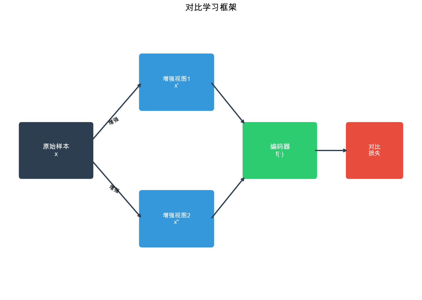
Contrastive Learning Framework

Contrastive learning is a specific type of SSL that learns by contrasting positive and negative pairs:

Core Principle: Pull similar examples (positives) together in embedding space, push dissimilar examples (negatives) apart.

Mathematically, given an anchor sample \(x\), a positive sample\(x^+\), and negative samples\(\{x_i^-\}_{i=1}^N\), contrastive learning optimizes:\[\mathcal{L}_{contrastive} = -\log \frac{\exp(\text{sim}(f(x), f(x^+)) / \tau)}{\exp(\text{sim}(f(x), f(x^+)) / \tau) + \sum_{i=1}^N \exp(\text{sim}(f(x), f(x_i^-)) / \tau)}\]where: -\(f(\cdot)\)is the encoder function -\(\text{sim}(\cdot, \cdot)\)is a similarity function (typically cosine similarity) -\(\tau\)is a temperature parameter controlling the concentration of the distribution

Key Components

1. Data Augmentation: Creating multiple views of the same data
   • For images: rotation, cropping, color jittering
   • For graphs: edge dropping, node masking
   • For sequences: item masking, reordering
2. Encoder Architecture: Neural network that maps inputs to embeddings
   • Should be expressive enough to capture complex patterns
   • Should be regularized to prevent collapse
3. Projection Head: Optional MLP that maps embeddings to contrastive space
   • Often improves performance by allowing the encoder to learn more general features
   • Typically discarded after training
4. Negative Sampling: Selecting negative examples
   • In-batch negatives: use other samples in the batch
   • Hard negatives: samples that are similar but should be different
   • Easy negatives: obviously different samples

InfoNCE Loss

The most common contrastive loss is InfoNCE (Information Noise Contrastive Estimation):\[\mathcal{L}_{InfoNCE} = -\mathbb{E} \left[ \log \frac{\exp(\text{sim}(z_i, z_j^+) / \tau)}{\sum_{k=1}^{2N} \mathbb{1}_{k \ne i} \exp(\text{sim}(z_i, z_k) / \tau)} \right]\]where: -\(z_i = f(x_i)\)is the embedding of anchor -\(z_j^+\)is the embedding of positive - The denominator includes all negatives in the batch -\(\mathbb{1}_{k \ne i}\)ensures we don't compare an anchor with itself

Why InfoNCE works: It maximizes the mutual information between positive pairs while minimizing it for negative pairs. This encourages the model to learn representations that capture the essential information needed to distinguish positives from negatives.

---

SimCLR: A Foundation for Contrastive Learning

SimCLR (Simple Contrastive Learning of Representations) introduced a simple yet powerful framework that became the foundation for many contrastive learning methods in recommendations.

SimCLR Architecture

SimCLR consists of four components:

1. Data Augmentation Module:\(\mathcal{T}\)

• applies random augmentations

2. Base Encoder:\(f(\cdot)\)

• extracts representations (e.g., ResNet)

3. Projection Head:\(g(\cdot)\)

• maps to contrastive space

4. Contrastive Loss: InfoNCE loss

Algorithm Overview

For each sample\(x\): 1. Generate two augmented views:\(\tilde{x}_i = t(x)\),\(\tilde{x}_j = t'(x)\)where\(t, t' \sim\)\(2. Encode:\)h_i = f(_i)\(,\)h_j = f(_j)\(3. Project:\)z_i = g(h_i)\(,\)z_j = g(h_j)\(4. Compute contrastive loss between\)z_i\(and\)z_j$

Key Design Choices

Large Batch Sizes: SimCLR requires large batches (4096+) because negatives come from other samples in the batch. Larger batches = more negatives = better learning signal.

Projection Head: A 2-layer MLP with ReLU activation significantly improves performance. The projection head can be discarded after training.

Strong Augmentations: SimCLR showed that stronger augmentations lead to better representations. The model learns to be invariant to these transformations.

Temperature Parameter:\(\tau = 0.07\)was found to work well. Lower temperatures make the distribution sharper (harder negatives matter more).

SimCLR Implementation for Recommendations

Here's how we can adapt SimCLR for recommendation systems:

import torch
import torch.nn as nn
import torch.nn.functional as F
from torch_geometric.nn import GCNConv
import numpy as np

class SimCLRRecommender(nn.Module):
    """
    SimCLR adapted for recommendation systems.
    Uses graph augmentation and contrastive learning.
    """
    def __init__(self, num_users, num_items, embedding_dim=64, 
                 hidden_dim=128, projection_dim=64, temperature=0.07):
        super(SimCLRRecommender, self).__init__()
        self.temperature = temperature
        
        # User and item embeddings
        self.user_embedding = nn.Embedding(num_users, embedding_dim)
        self.item_embedding = nn.Embedding(num_items, embedding_dim)
        
        # Encoder: MLP that processes user-item interactions
        self.encoder = nn.Sequential(
            nn.Linear(embedding_dim * 2, hidden_dim),
            nn.ReLU(),
            nn.Linear(hidden_dim, hidden_dim),
            nn.ReLU()
        )
        
        # Projection head
        self.projection = nn.Sequential(
            nn.Linear(hidden_dim, projection_dim),
            nn.ReLU(),
            nn.Linear(projection_dim, projection_dim)
        )
        
    def augment_graph(self, edge_index, drop_prob=0.2):
        """
        Graph augmentation: randomly drop edges.
        """
        if self.training:
            num_edges = edge_index.size(1)
            num_drop = int(num_edges * drop_prob)
            drop_indices = torch.randperm(num_edges)[:num_drop]
            mask = torch.ones(num_edges, dtype=torch.bool, device=edge_index.device)
            mask[drop_indices] = False
            return edge_index[:, mask]
        return edge_index
    
    def encode(self, user_ids, item_ids, edge_index):
        """
        Encode user-item pairs into representations.
        """
        # Get embeddings
        user_emb = self.user_embedding(user_ids)
        item_emb = self.item_embedding(item_ids)
        
        # Concatenate user and item embeddings
        pair_emb = torch.cat([user_emb, item_emb], dim=1)
        
        # Encode
        h = self.encoder(pair_emb)
        return h
    
    def forward(self, user_ids, item_ids, edge_index):
        """
        Forward pass with two augmented views.
        """
        # Create two augmented views
        edge_index_1 = self.augment_graph(edge_index, drop_prob=0.2)
        edge_index_2 = self.augment_graph(edge_index, drop_prob=0.2)
        
        # Encode both views
        h1 = self.encode(user_ids, item_ids, edge_index_1)
        h2 = self.encode(user_ids, item_ids, edge_index_2)
        
        # Project to contrastive space
        z1 = self.projection(h1)
        z2 = self.projection(h2)
        
        # Normalize
        z1 = F.normalize(z1, dim=1)
        z2 = F.normalize(z2, dim=1)
        
        return z1, z2
    
    def contrastive_loss(self, z1, z2):
        """
        Compute InfoNCE loss.
        """
        batch_size = z1.size(0)
        
        # Concatenate all embeddings
        z = torch.cat([z1, z2], dim=0)  # [2*B, D]
        
        # Create labels: positives are (i, i+B) pairs
        labels = torch.arange(batch_size, device=z.device)
        labels = torch.cat([labels + batch_size, labels], dim=0)
        
        # Compute similarity matrix
        sim_matrix = torch.matmul(z, z.T) / self.temperature
        
        # Mask out self-similarity
        mask = torch.eye(2 * batch_size, dtype=torch.bool, device=z.device)
        sim_matrix = sim_matrix.masked_fill(mask, float('-inf'))
        
        # For each sample, positive is its augmented pair
        # Negative is everything else in the batch
        labels = torch.arange(batch_size, device=z.device)
        labels = torch.cat([labels + batch_size, labels], dim=0)
        
        # Compute loss
        loss = F.cross_entropy(sim_matrix, labels)
        
        return loss

# Training example
def train_simclr(model, user_ids, item_ids, edge_index, optimizer):
    """
    Training loop for SimCLR recommender.
    """
    model.train()
    optimizer.zero_grad()
    
    # Forward pass
    z1, z2 = model(user_ids, item_ids, edge_index)
    
    # Compute contrastive loss
    loss = model.contrastive_loss(z1, z2)
    
    # Backward pass
    loss.backward()
    optimizer.step()
    
    return loss.item()

# Usage
num_users = 1000
num_items = 5000
model = SimCLRRecommender(num_users, num_items)
optimizer = torch.optim.Adam(model.parameters(), lr=0.001)

# Example training
for epoch in range(100):
    user_ids = torch.randint(0, num_users, (64,))
    item_ids = torch.randint(0, num_items, (64,))
    edge_index = torch.randint(0, num_users, (2, 1000))
    
    loss = train_simclr(model, user_ids, item_ids, edge_index, optimizer)
    if epoch % 10 == 0:
        print(f"Epoch {epoch}, Loss: {loss:.4f}")

Key Insights from SimCLR

1. Augmentation is Critical: The choice of augmentation strategy directly impacts what the model learns. For recommendations, this means carefully designing graph/sequence augmentations.

2. Projection Head Matters: The projection head allows the encoder to learn more general features while the projection learns task-specific representations.

3. Batch Size vs. Performance: Larger batches provide more negatives, improving the contrastive signal. However, this must be balanced with memory constraints.

4. Temperature Tuning: The temperature parameter is crucial. Too high (smooth distribution) or too low (sharp distribution) both hurt performance.

---

SGL: Self-Supervised Graph Learning for Recommendations

SGL (Self-supervised Graph Learning) adapts contrastive learning specifically for graph-based recommendation systems. It's one of the most influential methods for applying contrastive learning to recommendations.

Motivation

Graph Neural Networks (GNNs) have shown great success in recommendation systems by modeling user-item interactions as a bipartite graph. However, GNNs suffer from: - Data sparsity: Limited supervision signals - Over-smoothing: Node embeddings become too similar after many layers - Cold-start: New users/items have no connections

SGL addresses these by introducing self-supervised learning through graph augmentation.

SGL Architecture

SGL consists of three main components:

1. Graph Augmentation: Creates multiple views of the user-item graph
2. GNN Encoder: Extracts node representations from augmented graphs
3. Contrastive Learning: Trains encoder to be invariant to augmentations

Graph Augmentation Strategies

SGL proposes three augmentation strategies:

1. Node Dropout

Randomly masks out some nodes (users or items) and their associated edges:

def node_dropout(edge_index, node_mask, num_nodes):
    """
    Drop nodes and their associated edges.
    
    Args:
        edge_index: [2, E] edge tensor
        node_mask: [N] boolean mask (True = keep, False = drop)
        num_nodes: total number of nodes
    """
    # Filter edges where both endpoints are kept
    row, col = edge_index
    mask = node_mask[row] & node_mask[col]
    return edge_index[:, mask]

# Example
edge_index = torch.tensor([[0, 1, 2, 3], [4, 5, 6, 7]])  # 4 edges
node_mask = torch.tensor([True, False, True, True, True, False, True, True])
filtered_edges = node_dropout(edge_index, node_mask, 8)
# Only edges (0,4), (2,6), (3,7) remain

2. Edge Dropout

Randomly removes a fraction of edges:

def edge_dropout(edge_index, drop_prob=0.2):
    """
    Randomly drop edges.
    
    Args:
        edge_index: [2, E] edge tensor
        drop_prob: probability of dropping each edge
    """
    if not self.training:
        return edge_index
    
    num_edges = edge_index.size(1)
    num_drop = int(num_edges * drop_prob)
    drop_indices = torch.randperm(num_edges)[:num_drop]
    mask = torch.ones(num_edges, dtype=torch.bool, device=edge_index.device)
    mask[drop_indices] = False
    return edge_index[:, mask]

3. Random Walk

Generates subgraphs through random walks:

def random_walk_subgraph(edge_index, start_node, walk_length=10, 
                        return_prob=0.3, inout_prob=0.3):
    """
    Generate subgraph via random walk.
    
    Args:
        edge_index: [2, E] edge tensor
        start_node: starting node
        walk_length: length of random walk
        return_prob: probability of returning to previous node
        inout_prob: probability of staying in same node type
    """
    # Implementation of random walk with restart
    # Returns subgraph nodes and edges
    visited_nodes = {start_node}
    current_node = start_node
    
    for _ in range(walk_length):
        # Get neighbors
        neighbors = get_neighbors(edge_index, current_node)
        if len(neighbors) == 0:
            break
        
        # Random walk decision
        rand = np.random.random()
        if rand < return_prob and len(visited_nodes) > 1:
            # Return to previous node
            current_node = list(visited_nodes)[-2]
        elif rand < return_prob + inout_prob:
            # Stay in same node type (user or item)
            same_type_neighbors = filter_same_type(neighbors, current_node)
            if len(same_type_neighbors) > 0:
                current_node = np.random.choice(same_type_neighbors)
            else:
                current_node = np.random.choice(neighbors)
        else:
            # Random neighbor
            current_node = np.random.choice(neighbors)
        
        visited_nodes.add(current_node)
    
    # Extract subgraph
    subgraph_nodes = list(visited_nodes)
    subgraph_edges = extract_subgraph_edges(edge_index, subgraph_nodes)
    
    return subgraph_nodes, subgraph_edges

SGL Model Implementation

Here's a complete SGL implementation:

import torch
import torch.nn as nn
import torch.nn.functional as F
from torch_geometric.nn import LightGCNConv
from torch_geometric.utils import add_self_loops, degree

class SGLRecommender(nn.Module):
    """
    Self-Supervised Graph Learning for Recommendation.
    """
    def __init__(self, num_users, num_items, embedding_dim=64, 
                 num_layers=3, aug_type='edge', drop_prob=0.1):
        super(SGLRecommender, self).__init__()
        self.num_users = num_users
        self.num_items = num_items
        self.embedding_dim = embedding_dim
        self.num_layers = num_layers
        self.aug_type = aug_type
        self.drop_prob = drop_prob
        
        # Embeddings
        self.user_embedding = nn.Embedding(num_users, embedding_dim)
        self.item_embedding = nn.Embedding(num_items, embedding_dim)
        
        # Initialize embeddings
        nn.init.normal_(self.user_embedding.weight, std=0.1)
        nn.init.normal_(self.item_embedding.weight, std=0.1)
        
        # LightGCN layers
        self.convs = nn.ModuleList([
            LightGCNConv(embedding_dim, embedding_dim) 
            for _ in range(num_layers)
        ])
        
    def get_embeddings(self):
        """Get initial user and item embeddings."""
        return torch.cat([self.user_embedding.weight, 
                         self.item_embedding.weight], dim=0)
    
    def augment_graph(self, edge_index, num_nodes):
        """
        Apply graph augmentation.
        
        Args:
            edge_index: [2, E] edge tensor
            num_nodes: total number of nodes (users + items)
        """
        if not self.training:
            return edge_index
        
        if self.aug_type == 'edge':
            # Edge dropout
            num_edges = edge_index.size(1)
            num_drop = int(num_edges * self.drop_prob)
            drop_indices = torch.randperm(num_edges, device=edge_index.device)[:num_drop]
            mask = torch.ones(num_edges, dtype=torch.bool, device=edge_index.device)
            mask[drop_indices] = False
            return edge_index[:, mask]
        
        elif self.aug_type == 'node':
            # Node dropout
            node_mask = torch.rand(num_nodes, device=edge_index.device) > self.drop_prob
            row, col = edge_index
            mask = node_mask[row] & node_mask[col]
            return edge_index[:, mask]
        
        elif self.aug_type == 'mixed':
            # Randomly choose between edge and node dropout
            if torch.rand(1).item() < 0.5:
                return self.augment_graph(edge_index, num_nodes, 'edge')
            else:
                return self.augment_graph(edge_index, num_nodes, 'node')
        
        return edge_index
    
    def forward(self, edge_index, aug_edge_index=None):
        """
        Forward pass through GNN.
        
        Args:
            edge_index: original graph edges
            aug_edge_index: augmented graph edges (for contrastive learning)
        """
        # Get embeddings
        x = self.get_embeddings()
        num_nodes = x.size(0)
        
        # Use augmented graph if provided
        if aug_edge_index is not None:
            edge_index = aug_edge_index
        
        # Add self-loops
        edge_index, _ = add_self_loops(edge_index, num_nodes=num_nodes)
        
        # LightGCN propagation
        embeddings = [x]
        for conv in self.convs:
            x = conv(x, edge_index)
            embeddings.append(x)
        
        # Average embeddings from all layers
        final_embedding = torch.mean(torch.stack(embeddings), dim=0)
        
        return final_embedding
    
    def compute_contrastive_loss(self, z1, z2, temperature=0.2):
        """
        Compute contrastive loss between two views.
        
        Args:
            z1, z2: [N, D] node embeddings from two augmented views
            temperature: temperature parameter
        """
        # Normalize embeddings
        z1 = F.normalize(z1, dim=1)
        z2 = F.normalize(z2, dim=1)
        
        # Split into user and item embeddings
        user_emb_1 = z1[:self.num_users]
        user_emb_2 = z2[:self.num_users]
        item_emb_1 = z1[self.num_users:]
        item_emb_2 = z2[self.num_users:]
        
        # User-level contrastive loss
        user_sim = torch.matmul(user_emb_1, user_emb_2.T) / temperature
        user_labels = torch.arange(self.num_users, device=z1.device)
        user_loss = F.cross_entropy(user_sim, user_labels)
        
        # Item-level contrastive loss
        item_sim = torch.matmul(item_emb_1, item_emb_2.T) / temperature
        item_labels = torch.arange(self.num_items, device=z1.device)
        item_loss = F.cross_entropy(item_sim, item_labels)
        
        return user_loss + item_loss
    
    def predict(self, user_ids, item_ids, edge_index):
        """Predict ratings for user-item pairs."""
        embeddings = self.forward(edge_index)
        user_emb = embeddings[user_ids]
        item_emb = embeddings[self.num_users + item_ids]
        return torch.sum(user_emb * item_emb, dim=1)

# Training function
def train_sgl(model, edge_index, optimizer, alpha=0.1):
    """
    Train SGL model with contrastive learning.
    
    Args:
        model: SGL model
        edge_index: graph edges
        optimizer: optimizer
        alpha: weight for contrastive loss
    """
    model.train()
    optimizer.zero_grad()
    
    num_nodes = model.num_users + model.num_items
    
    # Create two augmented views
    aug_edge_index_1 = model.augment_graph(edge_index, num_nodes)
    aug_edge_index_2 = model.augment_graph(edge_index, num_nodes)
    
    # Forward pass for both views
    z1 = model.forward(edge_index, aug_edge_index_1)
    z2 = model.forward(edge_index, aug_edge_index_2)
    
    # Contrastive loss
    contrastive_loss = model.compute_contrastive_loss(z1, z2)
    
    # Recommendation loss (BPR or other)
    # Here we use a simple dot product loss
    # In practice, you'd use BPR loss with sampled negative items
    recommendation_loss = compute_recommendation_loss(model, edge_index)
    
    # Total loss
    total_loss = recommendation_loss + alpha * contrastive_loss
    
    total_loss.backward()
    optimizer.step()
    
    return total_loss.item(), contrastive_loss.item(), recommendation_loss.item()

def compute_recommendation_loss(model, edge_index):
    """
    Compute recommendation loss (e.g., BPR loss).
    This is a simplified version - in practice, you'd sample negatives.
    """
    # Get embeddings
    embeddings = model.forward(edge_index)
    user_emb = embeddings[:model.num_users]
    item_emb = embeddings[model.num_users:]
    
    # Sample positive and negative pairs
    row, col = edge_index
    user_ids = row[row < model.num_users]
    item_ids = col[col >= model.num_users] - model.num_users
    
    # Positive scores
    pos_scores = torch.sum(user_emb[user_ids] * item_emb[item_ids], dim=1)
    
    # Sample negative items
    neg_item_ids = torch.randint(0, model.num_items, 
                                (len(user_ids),), device=user_ids.device)
    neg_scores = torch.sum(user_emb[user_ids] * item_emb[neg_item_ids], dim=1)
    
    # BPR loss
    loss = -torch.log(torch.sigmoid(pos_scores - neg_scores) + 1e-10).mean()
    
    return loss

SGL Key Contributions

1. Graph-Specific Augmentations: SGL introduced augmentations tailored for bipartite graphs (node dropout, edge dropout) that preserve the graph structure while creating diverse views.

2. Multi-Level Contrastive Learning: SGL applies contrastive learning at both user and item levels, learning better representations for both entity types.

3. LightGCN Integration: SGL uses LightGCN as the base encoder, combining the benefits of GNNs with contrastive learning.

4. Empirical Success: SGL showed significant improvements over traditional GNN-based recommenders, especially for sparse data and cold-start scenarios.

---

RecDCL: Recommendation via Dual Contrastive Learning

RecDCL introduces dual contrastive learning, applying contrastive objectives at both the instance level and the prototype level.

Motivation

While SGL focuses on graph augmentation, RecDCL addresses a different challenge: learning both fine-grained instance representations and high-level prototype representations. This dual-level learning helps the model capture both local patterns (specific user-item interactions) and global patterns (user/item clusters).

Dual Contrastive Learning Framework

RecDCL applies contrastive learning at two levels:

1. Instance-Level Contrastive Learning: Similar to SGL, contrasts augmented views of the same instance
2. Prototype-Level Contrastive Learning: Contrasts prototypes (cluster centers) to learn better clustering

Architecture

import torch
import torch.nn as nn
import torch.nn.functional as F
from sklearn.cluster import KMeans

class RecDCL(nn.Module):
    """
    Recommendation via Dual Contrastive Learning.
    """
    def __init__(self, num_users, num_items, embedding_dim=64, 
                 num_prototypes=10, temperature=0.2):
        super(RecDCL, self).__init__()
        self.num_users = num_users
        self.num_items = num_items
        self.embedding_dim = embedding_dim
        self.num_prototypes = num_prototypes
        self.temperature = temperature
        
        # Embeddings
        self.user_embedding = nn.Embedding(num_users, embedding_dim)
        self.item_embedding = nn.Embedding(num_items, embedding_dim)
        
        # Prototype embeddings (learnable cluster centers)
        self.user_prototypes = nn.Parameter(
            torch.randn(num_prototypes, embedding_dim))
        self.item_prototypes = nn.Parameter(
            torch.randn(num_prototypes, embedding_dim))
        
    def forward(self, user_ids, item_ids, edge_index):
        """Forward pass."""
        user_emb = self.user_embedding(user_ids)
        item_emb = self.item_embedding(item_ids)
        return user_emb, item_emb
    
    def augment_embeddings(self, user_emb, item_emb, drop_prob=0.1):
        """
        Augment embeddings by adding noise or dropout.
        """
        if not self.training:
            return user_emb, item_emb
        
        # Add Gaussian noise
        user_noise = torch.randn_like(user_emb) * drop_prob
        item_noise = torch.randn_like(item_emb) * drop_prob
        
        user_emb_aug = user_emb + user_noise
        item_emb_aug = item_emb + item_noise
        
        return user_emb_aug, item_emb_aug
    
    def instance_contrastive_loss(self, z1, z2):
        """
        Instance-level contrastive loss.
        Similar to SGL's contrastive loss.
        """
        z1 = F.normalize(z1, dim=1)
        z2 = F.normalize(z2, dim=1)
        
        sim_matrix = torch.matmul(z1, z2.T) / self.temperature
        
        # Positive pairs are on the diagonal
        labels = torch.arange(z1.size(0), device=z1.device)
        loss = F.cross_entropy(sim_matrix, labels)
        
        return loss
    
    def prototype_contrastive_loss(self, embeddings, prototypes):
        """
        Prototype-level contrastive loss.
        Encourages embeddings to be close to their assigned prototypes.
        """
        embeddings = F.normalize(embeddings, dim=1)
        prototypes = F.normalize(prototypes, dim=1)
        
        # Assign embeddings to prototypes
        sim_to_prototypes = torch.matmul(embeddings, prototypes.T) / self.temperature
        
        # Soft assignment
        assignment = F.softmax(sim_to_prototypes, dim=1)
        
        # Contrastive loss: embeddings should be close to assigned prototype
        # and far from other prototypes
        loss = -torch.sum(assignment * torch.log(assignment + 1e-10))
        
        return loss
    
    def compute_dual_contrastive_loss(self, user_ids, item_ids, edge_index, 
                                      alpha=0.5, beta=0.5):
        """
        Compute dual contrastive loss.
        
        Args:
            alpha: weight for instance-level loss
            beta: weight for prototype-level loss
        """
        # Get embeddings
        user_emb, item_emb = self.forward(user_ids, item_ids, edge_index)
        
        # Augment embeddings
        user_emb_1, item_emb_1 = self.augment_embeddings(user_emb, item_emb)
        user_emb_2, item_emb_2 = self.augment_embeddings(user_emb, item_emb)
        
        # Instance-level contrastive loss
        user_instance_loss = self.instance_contrastive_loss(user_emb_1, user_emb_2)
        item_instance_loss = self.instance_contrastive_loss(item_emb_1, item_emb_2)
        instance_loss = user_instance_loss + item_instance_loss
        
        # Prototype-level contrastive loss
        user_proto_loss = self.prototype_contrastive_loss(
            user_emb, self.user_prototypes)
        item_proto_loss = self.prototype_contrastive_loss(
            item_emb, self.item_prototypes)
        proto_loss = user_proto_loss + item_proto_loss
        
        # Total loss
        total_loss = alpha * instance_loss + beta * proto_loss
        
        return total_loss, instance_loss, proto_loss

Key Insights from RecDCL

1. Dual-Level Learning: Learning at both instance and prototype levels helps capture hierarchical patterns in user-item interactions.

2. Prototype Learning: Prototypes act as learnable cluster centers, helping the model discover user/item groups automatically.

3. Complementary Objectives: Instance-level learning captures fine-grained patterns, while prototype-level learning captures coarse-grained patterns.

---

RCL: Robust Contrastive Learning

RCL (Robust Contrastive Learning) addresses the problem of noisy and adversarial examples in contrastive learning for recommendations.

The Robustness Problem

Real-world recommendation data contains: - Noisy interactions: Accidental clicks, bot traffic, mislabeled data - Adversarial examples: Users trying to game the system - Distribution shift: Training and test distributions differ

Standard contrastive learning is sensitive to these issues, leading to degraded performance.

RCL Approach

RCL makes contrastive learning robust by:

1. Robust Negative Sampling: Identifies and downweights hard negatives that might be false negatives
2. Adversarial Augmentation: Uses adversarial examples during training to improve robustness
3. Confidence Weighting: Weights contrastive losses by confidence scores

Implementation

class RCLRecommender(nn.Module):
    """
    Robust Contrastive Learning for Recommendation.
    """
    def __init__(self, num_users, num_items, embedding_dim=64, 
                 temperature=0.2, robust_weight=0.1):
        super(RCLRecommender, self).__init__()
        self.num_users = num_users
        self.num_items = num_items
        self.embedding_dim = embedding_dim
        self.temperature = temperature
        self.robust_weight = robust_weight
        
        # Embeddings
        self.user_embedding = nn.Embedding(num_users, embedding_dim)
        self.item_embedding = nn.Embedding(num_items, embedding_dim)
        
        # Confidence network (learns confidence scores)
        self.confidence_net = nn.Sequential(
            nn.Linear(embedding_dim, 32),
            nn.ReLU(),
            nn.Linear(32, 1),
            nn.Sigmoid()
        )
    
    def forward(self, user_ids, item_ids):
        """Forward pass."""
        user_emb = self.user_embedding(user_ids)
        item_emb = self.item_embedding(item_ids)
        return user_emb, item_emb
    
    def adversarial_augmentation(self, embeddings, epsilon=0.1):
        """
        Create adversarial examples by adding perturbations.
        """
        embeddings.requires_grad_(True)
        
        # Compute gradient of contrastive loss w.r.t. embeddings
        # (simplified - in practice, you'd compute full gradient)
        noise = torch.randn_like(embeddings) * epsilon
        return embeddings + noise
    
    def robust_contrastive_loss(self, z1, z2, confidence_scores):
        """
        Robust contrastive loss with confidence weighting.
        
        Args:
            z1, z2: embeddings from two views
            confidence_scores: [B] confidence scores for each sample
        """
        z1 = F.normalize(z1, dim=1)
        z2 = F.normalize(z2, dim=1)
        
        # Compute similarity matrix
        sim_matrix = torch.matmul(z1, z2.T) / self.temperature
        
        # Weight by confidence
        confidence_matrix = confidence_scores.unsqueeze(1) * confidence_scores.unsqueeze(0)
        weighted_sim = sim_matrix * confidence_matrix
        
        # Standard contrastive loss
        labels = torch.arange(z1.size(0), device=z1.device)
        loss = F.cross_entropy(weighted_sim, labels)
        
        return loss
    
    def compute_loss(self, user_ids, item_ids, edge_index):
        """Compute robust contrastive loss."""
        # Get embeddings
        user_emb, item_emb = self.forward(user_ids, item_ids)
        
        # Augment (standard)
        user_emb_1, item_emb_1 = self.augment_embeddings(user_emb, item_emb)
        user_emb_2, item_emb_2 = self.augment_embeddings(user_emb, item_emb)
        
        # Adversarial augmentation
        user_emb_adv = self.adversarial_augmentation(user_emb)
        item_emb_adv = self.adversarial_augmentation(item_emb)
        
        # Compute confidence scores
        user_conf = self.confidence_net(user_emb).squeeze()
        item_conf = self.confidence_net(item_emb).squeeze()
        
        # Robust contrastive loss
        user_loss = self.robust_contrastive_loss(
            user_emb_1, user_emb_2, user_conf)
        item_loss = self.robust_contrastive_loss(
            item_emb_1, item_emb_2, item_conf)
        
        # Adversarial loss
        adv_user_loss = self.robust_contrastive_loss(
            user_emb, user_emb_adv, user_conf)
        adv_item_loss = self.robust_contrastive_loss(
            item_emb, item_emb_adv, item_conf)
        
        total_loss = (user_loss + item_loss + 
                     self.robust_weight * (adv_user_loss + adv_item_loss))
        
        return total_loss

---

Advanced Graph Augmentation Strategies

Beyond simple edge/node dropout, several advanced augmentation strategies have been proposed for graph-based recommendations.

Adaptive Augmentation

Instead of random augmentation, adaptive methods learn which augmentations are most beneficial:

class AdaptiveGraphAugmentation(nn.Module):
    """
    Learn adaptive augmentation policies.
    """
    def __init__(self, num_nodes, embedding_dim=64):
        super(AdaptiveGraphAugmentation, self).__init__()
        self.num_nodes = num_nodes
        
        # Policy network: learns augmentation probabilities
        self.policy_net = nn.Sequential(
            nn.Linear(embedding_dim, 64),
            nn.ReLU(),
            nn.Linear(64, 1),
            nn.Sigmoid()
        )
    
    def adaptive_edge_dropout(self, edge_index, node_embeddings):
        """
        Adaptively drop edges based on learned policy.
        """
        row, col = edge_index
        
        # Compute edge importance scores
        edge_emb = node_embeddings[row] * node_embeddings[col]
        drop_probs = self.policy_net(edge_emb).squeeze()
        
        # Sample edges to drop
        keep_mask = torch.bernoulli(1 - drop_probs).bool()
        
        return edge_index[:, keep_mask]

Subgraph Sampling

Sample diverse subgraphs to create multiple views:

def subgraph_sampling(edge_index, num_nodes, num_samples=2, 
                     subgraph_size=1000):
    """
    Sample multiple subgraphs for contrastive learning.
    """
    subgraphs = []
    
    for _ in range(num_samples):
        # Random walk to get subgraph nodes
        start_node = torch.randint(0, num_nodes, (1,)).item()
        visited = {start_node}
        current = start_node
        
        # Random walk
        for _ in range(subgraph_size):
            neighbors = get_neighbors(edge_index, current)
            if len(neighbors) == 0:
                break
            current = np.random.choice(neighbors)
            visited.add(current)
        
        # Extract subgraph edges
        subgraph_nodes = list(visited)
        subgraph_edges = extract_subgraph_edges(edge_index, subgraph_nodes)
        subgraphs.append(subgraph_edges)
    
    return subgraphs

Feature Masking

For feature-rich graphs, mask node features:

def feature_masking(node_features, mask_prob=0.15):
    """
    Randomly mask node features (similar to BERT).
    """
    mask = torch.rand(node_features.size(0), device=node_features.device) > mask_prob
    masked_features = node_features.clone()
    masked_features[~mask] = 0  # or use learnable mask token
    return masked_features

---

XSimGCL: Simplified Graph Contrastive Learning

XSimGCL (eXtreme Simplified Graph Contrastive Learning) simplifies contrastive learning by removing the projection head and using cross-layer contrastive learning.

Key Innovation

XSimGCL makes two key simplifications:

1. No Projection Head: Directly contrasts embeddings from different GNN layers
2. Cross-Layer Contrastive Learning: Contrasts embeddings from different layers of the same view

Architecture

class XSimGCL(nn.Module):
    """
    eXtreme Simplified Graph Contrastive Learning.
    """
    def __init__(self, num_users, num_items, embedding_dim=64, 
                 num_layers=3, temperature=0.2):
        super(XSimGCL, self).__init__()
        self.num_users = num_users
        self.num_items = num_items
        self.embedding_dim = embedding_dim
        self.num_layers = num_layers
        self.temperature = temperature
        
        # Embeddings
        self.user_embedding = nn.Embedding(num_users, embedding_dim)
        self.item_embedding = nn.Embedding(num_items, embedding_dim)
        
        # GCN layers
        self.convs = nn.ModuleList([
            GCNConv(embedding_dim, embedding_dim) 
            for _ in range(num_layers)
        ])
    
    def forward(self, edge_index, aug_edge_index=None):
        """Forward pass."""
        x = torch.cat([self.user_embedding.weight, 
                      self.item_embedding.weight], dim=0)
        
        if aug_edge_index is not None:
            edge_index = aug_edge_index
        
        # Store embeddings from each layer
        layer_embeddings = [x]
        
        for conv in self.convs:
            x = conv(x, edge_index)
            x = F.relu(x)
            layer_embeddings.append(x)
        
        return layer_embeddings
    
    def cross_layer_contrastive_loss(self, layer_embeddings_1, layer_embeddings_2):
        """
        Contrast embeddings from different layers.
        """
        loss = 0
        
        # Contrast corresponding layers from two views
        for i in range(len(layer_embeddings_1)):
            z1 = F.normalize(layer_embeddings_1[i], dim=1)
            z2 = F.normalize(layer_embeddings_2[i], dim=1)
            
            # Positive pairs: same node, different views
            sim = torch.sum(z1 * z2, dim=1) / self.temperature
            loss += -torch.mean(sim)
        
        # Cross-layer contrastive: contrast different layers
        for i in range(len(layer_embeddings_1)):
            for j in range(i+1, len(layer_embeddings_1)):
                z_i = F.normalize(layer_embeddings_1[i], dim=1)
                z_j = F.normalize(layer_embeddings_1[j], dim=1)
                
                # Different layers should be similar (smoothness)
                sim = torch.sum(z_i * z_j, dim=1) / self.temperature
                loss += -torch.mean(sim) * 0.1  # Smaller weight
        
        return loss

Why XSimGCL Works

1. Simplicity: Removing the projection head reduces parameters and complexity
2. Layer Diversity: Cross-layer contrastive learning encourages smooth but diverse representations across layers
3. Efficiency: Fewer parameters and simpler architecture make training faster

---

Contrastive Learning for Sequential Recommendations

Sequential recommendation systems model user behavior as sequences of item interactions. Contrastive learning can be applied to learn better sequence representations.

Sequence Augmentation Strategies

For sequences, common augmentations include:

1. Item Masking: Randomly mask items in the sequence
2. Item Reordering: Shuffle non-adjacent items
3. Crop: Take a random subsequence
4. Insert: Insert random items

Implementation

class ContrastiveSequentialRecommender(nn.Module):
    """
    Contrastive learning for sequential recommendations.
    """
    def __init__(self, num_items, embedding_dim=64, hidden_dim=128, 
                 num_layers=2, temperature=0.2):
        super(ContrastiveSequentialRecommender, self).__init__()
        self.num_items = num_items
        self.embedding_dim = embedding_dim
        self.temperature = temperature
        
        # Item embeddings
        self.item_embedding = nn.Embedding(num_items, embedding_dim)
        
        # Sequence encoder (GRU or Transformer)
        self.encoder = nn.GRU(embedding_dim, hidden_dim, num_layers, 
                             batch_first=True)
        
        # Projection head
        self.projection = nn.Sequential(
            nn.Linear(hidden_dim, hidden_dim),
            nn.ReLU(),
            nn.Linear(hidden_dim, embedding_dim)
        )
    
    def augment_sequence(self, sequence, aug_type='mask'):
        """
        Augment sequence for contrastive learning.
        
        Args:
            sequence: [B, L] sequence of item IDs
            aug_type: 'mask', 'crop', 'reorder', or 'insert'
        """
        if aug_type == 'mask':
            # Randomly mask items
            mask_prob = 0.15
            mask = torch.rand(sequence.size(), device=sequence.device) > mask_prob
            augmented = sequence.clone()
            augmented[~mask] = 0  # 0 is mask token
            return augmented
        
        elif aug_type == 'crop':
            # Random crop
            seq_len = sequence.size(1)
            crop_len = int(seq_len * 0.8)
            start_idx = torch.randint(0, seq_len - crop_len + 1, (1,)).item()
            return sequence[:, start_idx:start_idx+crop_len]
        
        elif aug_type == 'reorder':
            # Shuffle non-adjacent items (preserve some order)
            # Simplified: just shuffle
            augmented = sequence.clone()
            for i in range(sequence.size(0)):
                perm = torch.randperm(sequence.size(1))
                augmented[i] = sequence[i][perm]
            return augmented
        
        return sequence
    
    def forward(self, sequence):
        """Encode sequence."""
        # Embed items
        item_emb = self.item_embedding(sequence)
        
        # Encode sequence
        output, hidden = self.encoder(item_emb)
        
        # Use last hidden state
        seq_emb = hidden[-1]  # [B, H]
        
        # Project
        z = self.projection(seq_emb)
        
        return z
    
    def contrastive_loss(self, z1, z2):
        """Compute contrastive loss."""
        z1 = F.normalize(z1, dim=1)
        z2 = F.normalize(z2, dim=1)
        
        sim_matrix = torch.matmul(z1, z2.T) / self.temperature
        
        labels = torch.arange(z1.size(0), device=z1.device)
        loss = F.cross_entropy(sim_matrix, labels)
        
        return loss
    
    def compute_loss(self, sequences):
        """Compute contrastive loss for sequences."""
        # Create two augmented views
        seq_1 = self.augment_sequence(sequences, 'mask')
        seq_2 = self.augment_sequence(sequences, 'crop')
        
        # Encode
        z1 = self.forward(seq_1)
        z2 = self.forward(seq_2)
        
        # Contrastive loss
        loss = self.contrastive_loss(z1, z2)
        
        return loss

Sequential Contrastive Learning Benefits

1. Temporal Invariance: Learns representations invariant to minor sequence variations
2. Better Generalization: Augmented sequences help model generalize to unseen patterns
3. Cold-Start: Better handling of short sequences (new users)

---

Contrastive Learning for Long-Tail Recommendations

Long-tail items (items with few interactions) are crucial for diversity but challenging to recommend. Contrastive learning can help by learning better representations for these items.

The Long-Tail Problem

In recommendation systems: - Head items (popular items) dominate interactions - Long-tail items (niche items) have few interactions but are important for diversity - Traditional models overfit to head items, ignoring long-tail

Contrastive Learning Solution

Contrastive learning helps by:

1. Learning from Structure: Even with few interactions, graph structure provides signal
2. Augmentation: Creates more training examples for long-tail items
3. Better Representations: Learns semantic similarity beyond interaction frequency

Implementation

class LongTailContrastiveRecommender(nn.Module):
    """
    Contrastive learning for long-tail recommendations.
    """
    def __init__(self, num_users, num_items, embedding_dim=64, 
                 temperature=0.2, tail_threshold=10):
        super(LongTailContrastiveRecommender, self).__init__()
        self.num_users = num_users
        self.num_items = num_items
        self.embedding_dim = embedding_dim
        self.temperature = temperature
        self.tail_threshold = tail_threshold  # Items with <10 interactions are long-tail
        
        # Embeddings
        self.user_embedding = nn.Embedding(num_users, embedding_dim)
        self.item_embedding = nn.Embedding(num_items, embedding_dim)
        
        # Separate embeddings for head and tail items
        self.tail_item_embedding = nn.Embedding(num_items, embedding_dim)
    
    def identify_tail_items(self, item_interaction_counts):
        """
        Identify long-tail items.
        
        Args:
            item_interaction_counts: [num_items] count of interactions per item
        """
        tail_mask = item_interaction_counts < self.tail_threshold
        return tail_mask
    
    def forward(self, user_ids, item_ids, is_tail=None):
        """Forward pass."""
        user_emb = self.user_embedding(user_ids)
        
        if is_tail is not None:
            # Use tail-specific embeddings for long-tail items
            item_emb = torch.where(
                is_tail.unsqueeze(1),
                self.tail_item_embedding(item_ids),
                self.item_embedding(item_ids)
            )
        else:
            item_emb = self.item_embedding(item_ids)
        
        return user_emb, item_emb
    
    def tail_aware_contrastive_loss(self, user_emb, item_emb, is_tail, 
                                    alpha=2.0):
        """
        Contrastive loss with higher weight for long-tail items.
        
        Args:
            alpha: weight multiplier for tail items
        """
        # Normalize embeddings
        user_emb = F.normalize(user_emb, dim=1)
        item_emb = F.normalize(item_emb, dim=1)
        
        # Compute similarities
        sim = torch.sum(user_emb * item_emb, dim=1) / self.temperature
        
        # Weight by tail status
        weights = torch.where(is_tail, 
                            torch.ones_like(is_tail) * alpha,
                            torch.ones_like(is_tail))
        
        # Contrastive loss (simplified)
        loss = -torch.mean(weights * torch.log(torch.sigmoid(sim) + 1e-10))
        
        return loss
    
    def compute_loss(self, user_ids, item_ids, item_interaction_counts):
        """Compute loss with long-tail awareness."""
        # Identify tail items
        tail_mask = self.identify_tail_items(item_interaction_counts)
        is_tail = tail_mask[item_ids]
        
        # Get embeddings
        user_emb, item_emb = self.forward(user_ids, item_ids, is_tail)
        
        # Augment
        user_emb_1, item_emb_1 = self.augment_embeddings(user_emb, item_emb)
        user_emb_2, item_emb_2 = self.augment_embeddings(user_emb, item_emb)
        
        # Contrastive loss with tail awareness
        loss_1 = self.tail_aware_contrastive_loss(
            user_emb_1, item_emb_1, is_tail)
        loss_2 = self.tail_aware_contrastive_loss(
            user_emb_2, item_emb_2, is_tail)
        
        return (loss_1 + loss_2) / 2

Key Strategies for Long-Tail

1. Tail-Specific Embeddings: Separate embedding spaces for head and tail items
2. Weighted Loss: Higher weight for long-tail items in contrastive loss
3. Graph Augmentation: More aggressive augmentation for tail items to create more training signals
4. Prototype Learning: Use prototypes to group similar tail items

---

Complete Training Pipeline

Here's a complete training pipeline that combines all the components:

import torch
import torch.nn as nn
import torch.optim as optim
from torch.utils.data import DataLoader, Dataset
import numpy as np
from sklearn.metrics import roc_auc_score, ndcg_score

class RecommendationDataset(Dataset):
    """Dataset for recommendation training."""
    def __init__(self, user_ids, item_ids, labels):
        self.user_ids = torch.LongTensor(user_ids)
        self.item_ids = torch.LongTensor(item_ids)
        self.labels = torch.FloatTensor(labels)
    
    def __len__(self):
        return len(self.user_ids)
    
    def __getitem__(self, idx):
        return self.user_ids[idx], self.item_ids[idx], self.labels[idx]

class CompleteContrastiveRecommender(nn.Module):
    """
    Complete contrastive learning recommender with all components.
    """
    def __init__(self, num_users, num_items, embedding_dim=64, 
                 num_layers=3, temperature=0.2, aug_type='edge', 
                 drop_prob=0.1):
        super(CompleteContrastiveRecommender, self).__init__()
        self.num_users = num_users
        self.num_items = num_items
        self.embedding_dim = embedding_dim
        self.temperature = temperature
        self.aug_type = aug_type
        self.drop_prob = drop_prob
        
        # Embeddings
        self.user_embedding = nn.Embedding(num_users, embedding_dim)
        self.item_embedding = nn.Embedding(num_items, embedding_dim)
        
        # GNN layers
        self.convs = nn.ModuleList([
            LightGCNConv(embedding_dim, embedding_dim) 
            for _ in range(num_layers)
        ])
        
        # Projection head
        self.projection = nn.Sequential(
            nn.Linear(embedding_dim, embedding_dim),
            nn.ReLU(),
            nn.Linear(embedding_dim, embedding_dim)
        )
    
    def get_embeddings(self):
        """Get initial embeddings."""
        return torch.cat([self.user_embedding.weight, 
                         self.item_embedding.weight], dim=0)
    
    def augment_graph(self, edge_index, num_nodes):
        """Augment graph."""
        if not self.training:
            return edge_index
        
        if self.aug_type == 'edge':
            num_edges = edge_index.size(1)
            num_drop = int(num_edges * self.drop_prob)
            drop_indices = torch.randperm(num_edges, device=edge_index.device)[:num_drop]
            mask = torch.ones(num_edges, dtype=torch.bool, device=edge_index.device)
            mask[drop_indices] = False
            return edge_index[:, mask]
        
        elif self.aug_type == 'node':
            node_mask = torch.rand(num_nodes, device=edge_index.device) > self.drop_prob
            row, col = edge_index
            mask = node_mask[row] & node_mask[col]
            return edge_index[:, mask]
        
        return edge_index
    
    def forward(self, edge_index, use_projection=False):
        """Forward pass."""
        x = self.get_embeddings()
        num_nodes = x.size(0)
        
        # Add self-loops
        edge_index, _ = add_self_loops(edge_index, num_nodes=num_nodes)
        
        # GNN propagation
        embeddings = [x]
        for conv in self.convs:
            x = conv(x, edge_index)
            embeddings.append(x)
        
        # Average embeddings
        final_embedding = torch.mean(torch.stack(embeddings), dim=0)
        
        # Projection
        if use_projection:
            final_embedding = self.projection(final_embedding)
        
        return final_embedding
    
    def compute_contrastive_loss(self, z1, z2):
        """Compute contrastive loss."""
        z1 = F.normalize(z1, dim=1)
        z2 = F.normalize(z2, dim=1)
        
        # Split user and item embeddings
        user_emb_1 = z1[:self.num_users]
        user_emb_2 = z2[:self.num_users]
        item_emb_1 = z1[self.num_users:]
        item_emb_2 = z2[self.num_users:]
        
        # User contrastive loss
        user_sim = torch.matmul(user_emb_1, user_emb_2.T) / self.temperature
        user_labels = torch.arange(self.num_users, device=z1.device)
        user_loss = F.cross_entropy(user_sim, user_labels)
        
        # Item contrastive loss
        item_sim = torch.matmul(item_emb_1, item_emb_2.T) / self.temperature
        item_labels = torch.arange(self.num_items, device=z1.device)
        item_loss = F.cross_entropy(item_sim, item_labels)
        
        return user_loss + item_loss
    
    def predict(self, user_ids, item_ids, edge_index):
        """Predict ratings."""
        embeddings = self.forward(edge_index, use_projection=False)
        user_emb = embeddings[user_ids]
        item_emb = embeddings[self.num_users + item_ids]
        return torch.sum(user_emb * item_emb, dim=1)

def train_contrastive_recommender(model, train_loader, edge_index, 
                                 optimizer, device, alpha=0.1):
    """
    Training function for contrastive recommender.
    
    Args:
        model: contrastive recommender model
        train_loader: data loader for training
        edge_index: graph edges
        optimizer: optimizer
        device: device
        alpha: weight for contrastive loss
    """
    model.train()
    total_loss = 0
    total_contrastive_loss = 0
    total_recommendation_loss = 0
    
    num_nodes = model.num_users + model.num_items
    
    for batch_idx, (user_ids, item_ids, labels) in enumerate(train_loader):
        user_ids = user_ids.to(device)
        item_ids = item_ids.to(device)
        labels = labels.to(device)
        
        optimizer.zero_grad()
        
        # Create two augmented views
        aug_edge_index_1 = model.augment_graph(edge_index, num_nodes)
        aug_edge_index_2 = model.augment_graph(edge_index, num_nodes)
        
        # Forward pass for both views
        z1 = model.forward(aug_edge_index_1, use_projection=True)
        z2 = model.forward(aug_edge_index_2, use_projection=True)
        
        # Contrastive loss
        contrastive_loss = model.compute_contrastive_loss(z1, z2)
        
        # Recommendation loss (BPR)
        embeddings = model.forward(edge_index, use_projection=False)
        user_emb = embeddings[user_ids]
        item_emb = embeddings[model.num_users + item_ids]
        
        # Positive scores
        pos_scores = torch.sum(user_emb * item_emb, dim=1)
        
        # Sample negative items
        neg_item_ids = torch.randint(0, model.num_items, 
                                    (len(user_ids),), device=device)
        neg_item_emb = embeddings[model.num_users + neg_item_ids]
        neg_scores = torch.sum(user_emb * neg_item_emb, dim=1)
        
        # BPR loss
        recommendation_loss = -torch.log(
            torch.sigmoid(pos_scores - neg_scores) + 1e-10).mean()
        
        # Total loss
        loss = recommendation_loss + alpha * contrastive_loss
        
        loss.backward()
        optimizer.step()
        
        total_loss += loss.item()
        total_contrastive_loss += contrastive_loss.item()
        total_recommendation_loss += recommendation_loss.item()
    
    return (total_loss / len(train_loader),
            total_contrastive_loss / len(train_loader),
            total_recommendation_loss / len(train_loader))

def evaluate(model, test_loader, edge_index, device):
    """Evaluate model."""
    model.eval()
    predictions = []
    labels = []
    
    with torch.no_grad():
        embeddings = model.forward(edge_index, use_projection=False)
        
        for user_ids, item_ids, label in test_loader:
            user_ids = user_ids.to(device)
            item_ids = item_ids.to(device)
            
            user_emb = embeddings[user_ids]
            item_emb = embeddings[model.num_users + item_ids]
            
            scores = torch.sum(user_emb * item_emb, dim=1)
            
            predictions.extend(scores.cpu().numpy())
            labels.extend(label.numpy())
    
    # Compute metrics
    auc = roc_auc_score(labels, predictions)
    
    return auc

# Example usage
def main():
    # Hyperparameters
    num_users = 1000
    num_items = 5000
    embedding_dim = 64
    num_layers = 3
    batch_size = 256
    learning_rate = 0.001
    num_epochs = 100
    alpha = 0.1  # Contrastive loss weight
    
    # Device
    device = torch.device('cuda' if torch.cuda.is_available() else 'cpu')
    
    # Model
    model = CompleteContrastiveRecommender(
        num_users, num_items, embedding_dim, num_layers
    ).to(device)
    
    # Optimizer
    optimizer = optim.Adam(model.parameters(), lr=learning_rate)
    
    # Data (example)
    # In practice, load from your dataset
    train_user_ids = np.random.randint(0, num_users, 10000)
    train_item_ids = np.random.randint(0, num_items, 10000)
    train_labels = np.random.randint(0, 2, 10000)
    
    train_dataset = RecommendationDataset(
        train_user_ids, train_item_ids, train_labels)
    train_loader = DataLoader(train_dataset, batch_size=batch_size, shuffle=True)
    
    # Graph edges (example)
    edge_index = torch.randint(0, num_users, (2, 5000)).to(device)
    
    # Training loop
    for epoch in range(num_epochs):
        loss, contrastive_loss, recommendation_loss = train_contrastive_recommender(
            model, train_loader, edge_index, optimizer, device, alpha)
        
        if epoch % 10 == 0:
            print(f"Epoch {epoch}: Total Loss={loss:.4f}, "
                  f"Contrastive={contrastive_loss:.4f}, "
                  f"Recommendation={recommendation_loss:.4f}")
    
    print("Training complete!")

if __name__ == "__main__":
    main()

---

Frequently Asked Questions (Q&A)

Q1: Why do we need contrastive learning for recommendations? Can't we just use more data?

A: While more data helps, contrastive learning provides several advantages beyond just data quantity:

1. Better Representations: Contrastive learning learns representations that capture semantic similarity, not just interaction patterns. This helps with generalization and cold-start scenarios.

2. Data Efficiency: Contrastive learning can achieve similar performance with less labeled data by leveraging self-supervision signals from data augmentation.

3. Robustness: Models trained with contrastive learning are more robust to noise and missing data, which is common in real-world recommendation scenarios.

4. Long-Tail Discovery: Contrastive learning helps discover and recommend long-tail items that traditional methods often ignore.

Q2: How do I choose the right augmentation strategy for my recommendation system?

A: The choice depends on your data type and problem:

• Graph-based (user-item interactions): Use edge dropout, node dropout, or subgraph sampling (like SGL)
• Sequential (user behavior sequences): Use item masking, sequence cropping, or reordering
• Feature-rich: Use feature masking or feature dropout
• Hybrid: Combine multiple augmentation strategies

Best Practice: Start with simple augmentations (edge dropout for graphs, masking for sequences) and experiment. Monitor validation performance to find what works best for your specific dataset.

Q3: What's the difference between SimCLR, SGL, and XSimGCL? Which should I use?

A:

• SimCLR: General contrastive learning framework, originally for images. Requires adaptation for recommendations. Good starting point for understanding contrastive learning.

• SGL: Specifically designed for graph-based recommendations. Uses graph augmentations (edge/node dropout) and LightGCN. Best for bipartite graph recommendation scenarios.

• XSimGCL: Simplified version that removes projection head and uses cross-layer contrastive learning. More efficient and often performs similarly to SGL.

Recommendation: Start with SGL if you have graph-structured data. Use XSimGCL if you want a simpler, more efficient model. Use SimCLR as a reference for understanding contrastive learning principles.

Q4: How do I set the temperature parameter\(\tau\)?

A: The temperature parameter controls the concentration of the similarity distribution:

• Low\(\tau\)(0.05-0.1): Sharper distribution, harder negatives matter more. Can be too aggressive.
• Medium\(\tau\)(0.1-0.2): Balanced, works well for most cases. Common default: 0.2.
• High\(\tau\)(0.5+): Softer distribution, easier negatives also contribute. May hurt performance.

Best Practice: Start with\(\tau = 0.2\)and tune based on validation performance. Lower values often work better for fine-grained distinctions, higher values for coarse-grained.

Q5: Do I need a projection head? When should I use it?

A: The projection head is an MLP that maps encoder outputs to contrastive space:

With Projection Head (SimCLR, SGL): - Allows encoder to learn more general features - Projection learns task-specific representations - Typically discarded after training - Usually improves performance

Without Projection Head (XSimGCL): - Simpler architecture - Fewer parameters - Direct contrastive learning on embeddings - Can work well if embeddings are already well-structured

Recommendation: Use a projection head unless you have strong reasons not to (e.g., efficiency constraints). It's a simple addition that often improves performance.

Q6: How do I handle negative sampling in contrastive learning?

A: Negative sampling strategies:

1. In-Batch Negatives: Use other samples in the batch as negatives. Simple and efficient, but requires large batches.

2. Hard Negatives: Samples that are similar but should be different. More informative but harder to identify.

3. Easy Negatives: Obviously different samples. Less informative but stable.

4. Mixed Strategy: Combine easy and hard negatives.

Best Practice: Start with in-batch negatives (simplest). For better performance, add hard negatives by sampling items similar to positive items but not interacted with.

Q7: Can contrastive learning work with implicit feedback (clicks, views) or do I need explicit ratings?

A: Contrastive learning works excellently with implicit feedback! In fact, it's often more suitable than explicit ratings because:

• Implicit feedback is more abundant (every click is a signal)
• Contrastive learning doesn't require exact ratings, just positive/negative pairs
• Graph structure from implicit interactions provides rich self-supervision signals

Most contrastive recommendation methods (SGL, XSimGCL) are designed for implicit feedback scenarios.

Q8: How do I combine contrastive learning with traditional recommendation losses (BPR, NCF)?

A: The standard approach is multi-task learning:\[\mathcal{L}_{total} = \mathcal{L}_{recommendation} + \alpha \cdot \mathcal{L}_{contrastive}\]where\(\alpha\)controls the weight of contrastive loss.

Example:

# Recommendation loss (BPR)
recommendation_loss = compute_bpr_loss(user_emb, pos_item_emb, neg_item_emb)

# Contrastive loss
contrastive_loss = compute_contrastive_loss(z1, z2)

# Total loss
total_loss = recommendation_loss + alpha * contrastive_loss

Tuning\(\alpha\): Start with\(\alpha = 0.1\)and adjust based on validation performance. Too high (\(>1.0\)) may hurt recommendation performance, too low (\(<0.01\)) may not help.

Q9: How much data do I need for contrastive learning to be effective?

A: Contrastive learning is more data-efficient than supervised learning, but still benefits from more data:

• Minimum: A few thousand user-item interactions
• Good Performance: 10K-100K interactions
• Excellent Performance: 100K+ interactions

However, contrastive learning can work with less data than pure supervised methods because: - Augmentation creates more training examples - Self-supervision signals don't require explicit labels - Graph structure provides additional signal

Key: Even with limited data, contrastive learning often outperforms traditional methods, especially for cold-start scenarios.

Q10: How do I evaluate contrastive learning models? Are standard metrics (AUC, NDCG) sufficient?

A: Standard metrics are still relevant, but consider additional evaluations:

Standard Metrics: - AUC/ROC: Overall ranking quality - NDCG@K: Top-K recommendation quality - Recall@K: Coverage of relevant items - Precision@K: Accuracy of top-K recommendations

Contrastive-Specific Evaluations: - Cold-Start Performance: Test on new users/items - Long-Tail Discovery: Measure recommendation diversity - Representation Quality: Visualize embeddings (t-SNE, UMAP) - Robustness: Test with noisy/missing data

Best Practice: Use standard metrics for comparison with baselines, but also evaluate cold-start and long-tail performance where contrastive learning shines.

Q11: Can I use contrastive learning for multi-modal recommendations (text, images, etc.)?

A: Yes! Contrastive learning is excellent for multi-modal scenarios:

Cross-Modal Contrastive Learning: - Contrast text and image representations of the same item - Learn aligned embeddings across modalities - Handle missing modalities gracefully

Example: For an item with both image and text, create positive pairs from the same item's modalities, negatives from different items.

Implementation: Use separate encoders for each modality, contrast embeddings in shared space.

Q12: How do I handle the computational cost of contrastive learning?

A: Contrastive learning can be computationally expensive. Optimization strategies:

1. Smaller Batches: Use gradient accumulation if memory is limited
2. Fewer Negatives: Limit negative sampling instead of using all in-batch negatives
3. Simpler Architecture: Use XSimGCL instead of SGL if needed
4. Efficient Augmentation: Cache augmented graphs instead of recomputing
5. Mixed Precision Training: Use FP16 to reduce memory and speed up training

Trade-off: Some performance loss may occur, but contrastive learning often still outperforms non-contrastive methods even with these optimizations.

---

Conclusion

Contrastive learning has emerged as a powerful paradigm for recommendation systems, addressing fundamental challenges like data sparsity, cold-start problems, and long-tail item discovery. By learning from data structure rather than relying solely on explicit labels, contrastive methods achieve better generalization and robustness.

Key takeaways:

1. Self-Supervision is Powerful: Learning from data structure provides rich signals even with limited labeled data.

2. Augmentation Matters: The choice of augmentation strategy directly impacts what the model learns. Graph augmentations (edge/node dropout) work well for recommendation graphs.

3. Simplicity Can Win: Methods like XSimGCL show that simpler architectures can match or exceed complex ones.

4. Multi-Level Learning: Combining instance-level and prototype-level contrastive learning (like RecDCL) captures both fine-grained and coarse-grained patterns.

5. Practical Impact: Contrastive learning provides significant improvements in cold-start scenarios, long-tail discovery, and overall recommendation diversity.

As recommendation systems continue to evolve, contrastive learning will likely play an increasingly important role. The methods we've covered — SimCLR, SGL, RecDCL, RCL, XSimGCL — represent the current state of the art, but the field is rapidly advancing. New techniques for better augmentations, more efficient training, and improved robustness are constantly being developed.

Whether you're building a new recommendation system or improving an existing one, understanding and applying contrastive learning is essential. Start with simple augmentations and standard methods like SGL, then experiment with more advanced techniques based on your specific needs and constraints.

The future of recommendation systems lies in learning better representations, and contrastive learning provides a powerful framework for achieving that goal.