Recommendation Systems (10): Deep Interest Networks and Attention Mechanisms

permalink: "en/recommendation-systems-10-deep-interest-networks/" date: 2024-06-16 15:15:00 tags: - Recommendation Systems - DIN - Attention Mechanism categories: Recommendation Systems mathjax: true--- When you browse Alibaba's e-commerce platform, the recommendation system doesn't treat all your past clicks equally. That vintage leather jacket you viewed last week matters more when you're looking at similar jackets today than the random phone charger you clicked months ago. This selective focus — understanding which historical behaviors are relevant to the current recommendation — is the core insight behind Deep Interest Networks (DIN), a breakthrough architecture that introduced attention mechanisms to recommendation systems and revolutionized how we model user interests.

Traditional recommendation models treat user behavior sequences as fixed-length vectors, averaging or pooling all historical interactions regardless of their relevance to the current item. DIN changed this paradigm by introducing target attention: dynamically weighting historical behaviors based on their similarity to the candidate item. This simple but powerful idea, combined with Alibaba's massive scale (billions of users, millions of items, terabytes of daily data), led to significant improvements in click-through rates and revenue. The success of DIN spawned a family of attention-based architectures: DIEN (Deep Interest Evolution Network) models how interests evolve over time, DSIN (Deep Session Interest Network) captures session-level patterns, and various attention variants address different aspects of the recommendation problem.

This article provides a comprehensive exploration of Deep Interest Networks and attention mechanisms in recommendation systems, covering the theoretical foundations of attention, DIN's target attention mechanism, DIEN's interest evolution modeling, DSIN's session-aware architecture, attention variants (multi-head, self-attention, co-attention), Alibaba's production practices and optimizations, training techniques for large-scale systems, and practical implementations with 10+ code examples and detailed Q&A sections addressing common questions and challenges.

The Attention Revolution in Recommendation Systems

Why Attention Matters

Traditional recommendation models face a fundamental limitation: they treat all historical user behaviors as equally important. Consider a user who has clicked on: - 5 action movies - 3 romantic comedies
- 2 documentaries - 1 horror film

When recommending a new action movie, the system should emphasize those 5 action movie clicks, not treat them equally with the horror film click. This selective focus is exactly what attention mechanisms provide.

The Core Problem

Given a user's behavior sequence\(\mathbf{B}_u = [b_1, b_2, \dots, b_T]\)where each\(b_i\)represents a historical interaction (click, purchase, view), and a candidate item\(i\), traditional models compute:\[\mathbf{v}_u = \text{Pool}(\mathbf{B}_u) = \frac{1}{T} \sum_{j=1}^{T} \mathbf{e}_{b_j}\]where\(\mathbf{e}_{b_j}\)is the embedding of behavior\(b_j\). This averaging loses the relevance information — all behaviors contribute equally regardless of how similar they are to the candidate item.

Attention Solution

Attention mechanisms compute a relevance score\(\alpha_j\)for each historical behavior\(b_j\)with respect to the candidate item\(i\):\[\alpha_j = \text{Attention}(\mathbf{e}_{b_j}, \mathbf{e}_i)\]The user representation becomes a weighted sum:\[\mathbf{v}_u = \sum_{j=1}^{T} \alpha_j \mathbf{e}_{b_j}\]where behaviors similar to the candidate item receive higher weights, allowing the model to focus on relevant historical patterns.

Attention Mechanism Fundamentals

Basic Attention

The attention mechanism computes a compatibility score between a query\(\mathbf{q}\)and a set of keys\(\mathbf{K} = [\mathbf{k}_1, \mathbf{k}_2, \dots, \mathbf{k}_n]\):\[\text{Attention}(\mathbf{q}, \mathbf{K}, \mathbf{V}) = \sum_{i=1}^{n} \alpha_i \mathbf{v}_i\]where the attention weights\(\alpha_i\)are computed as:\[\alpha_i = \frac{\exp(\text{score}(\mathbf{q}, \mathbf{k}_i))}{\sum_{j=1}^{n} \exp(\text{score}(\mathbf{q}, \mathbf{k}_j))}\]Common scoring functions include:

1. Dot-product attention:\(\text{score}(\mathbf{q}, \mathbf{k}_i) = \mathbf{q}^T \mathbf{k}_i\)

2. Scaled dot-product:\(\text{score}(\mathbf{q}, \mathbf{k}_i) = \frac{\mathbf{q}^T \mathbf{k}_i}{\sqrt{d }}\)

3. Additive attention:\(\text{score}(\mathbf{q}, \mathbf{k}_i) = \mathbf{v}^T \tanh(\mathbf{W}_q \mathbf{q} + \mathbf{W}_k \mathbf{k}_i)\) Target Attention in Recommendation

In recommendation systems, we use target attention (also called query attention), where: - Query: candidate item embedding\(\mathbf{e}_i\) - Keys: historical behavior embeddings\(\mathbf{e}_{b_j}\) - Values: historical behavior embeddings\(\mathbf{e}_{b_j}\)(self-attention)

The attention weight measures how relevant each historical behavior is to the current candidate item.

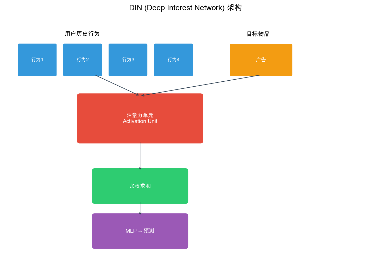
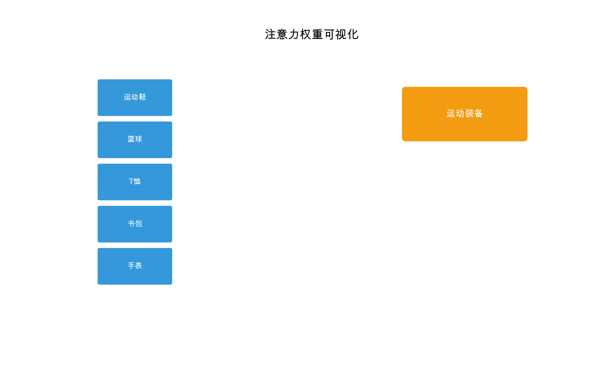
Deep Interest Network (DIN)

Architecture Overview

DIN was introduced by Alibaba in 2018 to address the limitation of fixed-length user representations in CTR prediction. The key innovation is the Local Activation Unit that adaptively computes attention weights based on the candidate item.

Problem Formulation

Given: - User profile features:\(\mathbf{x}_u\)(age, gender, city, etc.) - User behavior sequence:\(\mathbf{B}_u = [b_1, b_2, \dots, b_T]\)(clicked items) - Candidate item:\(i\)with features\(\mathbf{x}_i\) - Context features:\(\mathbf{x}_c\)(time, device, etc.)

Predict: CTR\(P(\text{click} | \mathbf{x}_u, \mathbf{B}_u, \mathbf{x}_i, \mathbf{x}_c)\) DIN Architecture

User Features → Embedding Layer
Behavior Sequence → Embedding Layer → Local Activation Unit (Attention)
Candidate Item → Embedding Layer
Context Features → Embedding Layer
                    ↓
            Concatenate All Features
                    ↓
            MLP Layers
                    ↓
            Output (CTR)

Local Activation Unit

The Local Activation Unit computes attention weights for each behavior in the sequence:\[\alpha_j = \text{Attention}(\mathbf{e}_{b_j}, \mathbf{e}_i) = \frac{\exp(\text{score}(\mathbf{e}_{b_j}, \mathbf{e}_i))}{\sum_{k=1}^{T} \exp(\text{score}(\mathbf{e}_{b_k}, \mathbf{e}_i))}\]The scoring function uses an MLP:\[\text{score}(\mathbf{e}_{b_j}, \mathbf{e}_i) = \mathbf{W}^T \text{ReLU}(\mathbf{W}_1 \mathbf{e}_{b_j} + \mathbf{W}_2 \mathbf{e}_i + \mathbf{b}) + c\]The activated user representation is:\[\mathbf{v}_u = \sum_{j=1}^{T} \alpha_j \mathbf{e}_{b_j}\]

Key Properties

1. Adaptive: Attention weights change based on the candidate item
2. Sparse: Only relevant behaviors get high weights
3. Interpretable: Attention weights show which behaviors matter

Implementation Example

import torch
import torch.nn as nn
import torch.nn.functional as F

class LocalActivationUnit(nn.Module):
    """Local Activation Unit for DIN"""
    
    def __init__(self, embedding_dim, hidden_dim=64):
        super(LocalActivationUnit, self).__init__()
        self.embedding_dim = embedding_dim
        
        # MLP for computing attention scores
        self.fc1 = nn.Linear(embedding_dim * 2, hidden_dim)
        self.fc2 = nn.Linear(hidden_dim, 1)
        
    def forward(self, behavior_embeddings, candidate_embedding):
        """
        Args:
            behavior_embeddings: [batch_size, seq_len, embedding_dim]
            candidate_embedding: [batch_size, embedding_dim]
        Returns:
            activated_user_embedding: [batch_size, embedding_dim]
            attention_weights: [batch_size, seq_len]
        """
        batch_size, seq_len, emb_dim = behavior_embeddings.shape
        
        # Expand candidate embedding to match sequence length
        candidate_expanded = candidate_embedding.unsqueeze(1).expand(
            batch_size, seq_len, emb_dim
        )
        
        # Concatenate behavior and candidate embeddings
        concat_features = torch.cat(
            [behavior_embeddings, candidate_expanded], dim=-1
        )
        
        # Compute attention scores
        attention_scores = self.fc2(
            F.relu(self.fc1(concat_features))
        ).squeeze(-1)  # [batch_size, seq_len]
        
        # Apply softmax to get attention weights
        attention_weights = F.softmax(attention_scores, dim=1)
        
        # Weighted sum of behavior embeddings
        activated_user_embedding = torch.sum(
            attention_weights.unsqueeze(-1) * behavior_embeddings,
            dim=1
        )
        
        return activated_user_embedding, attention_weights


class DIN(nn.Module):
    """Deep Interest Network"""
    
    def __init__(
        self,
        item_embedding_dim=64,
        user_feature_dim=32,
        context_feature_dim=16,
        hidden_dims=[200, 80],
        dropout=0.5
    ):
        super(DIN, self).__init__()
        
        self.item_embedding_dim = item_embedding_dim
        self.local_activation = LocalActivationUnit(
            item_embedding_dim, hidden_dim=64
        )
        
        # MLP layers
        mlp_input_dim = (
            item_embedding_dim +  # activated user embedding
            item_embedding_dim +  # candidate item embedding
            user_feature_dim +    # user profile features
            context_feature_dim    # context features
        )
        
        mlp_layers = []
        input_dim = mlp_input_dim
        for hidden_dim in hidden_dims:
            mlp_layers.append(nn.Linear(input_dim, hidden_dim))
            mlp_layers.append(nn.ReLU())
            mlp_layers.append(nn.Dropout(dropout))
            input_dim = hidden_dim
        
        mlp_layers.append(nn.Linear(input_dim, 1))
        mlp_layers.append(nn.Sigmoid())
        
        self.mlp = nn.Sequential(*mlp_layers)
        
    def forward(
        self,
        user_features,
        behavior_sequence,
        candidate_item,
        context_features
    ):
        """
        Args:
            user_features: [batch_size, user_feature_dim]
            behavior_sequence: [batch_size, seq_len, item_embedding_dim]
            candidate_item: [batch_size, item_embedding_dim]
            context_features: [batch_size, context_feature_dim]
        Returns:
            ctr: [batch_size, 1]
            attention_weights: [batch_size, seq_len]
        """
        # Local activation
        activated_user_embedding, attention_weights = self.local_activation(
            behavior_sequence, candidate_item
        )
        
        # Concatenate all features
        concat_features = torch.cat([
            activated_user_embedding,
            candidate_item,
            user_features,
            context_features
        ], dim=1)
        
        # MLP to predict CTR
        ctr = self.mlp(concat_features)
        
        return ctr, attention_weights

Training DIN

Loss Function

DIN uses binary cross-entropy loss for CTR prediction:\[\mathcal{L} = -\frac{1}{N} \sum_{i=1}^{N} [y_i \log(\hat{y}_i) + (1-y_i) \log(1-\hat{y}_i)]\]where\(y_i \in \{0, 1\}\)is the true label (click or not) and\(\hat{y}_i\)is the predicted CTR.

Mini-batch Aware Regularization

For large-scale training with millions of items, DIN uses mini-batch aware regularization for embedding layers:\[\mathcal{L}_{reg} = \sum_{j=1}^{K} \sum_{m=1}^{B} \frac{\alpha_{mj }}{n_j} ||\mathbf{e}_j||^2\]where: -\(K\)is the number of embedding tables -\(B\)is the number of mini-batches -\(\alpha_{mj}\)is the number of times feature\(j\)appears in batch\(m\) -\(n_j\)is the total frequency of feature\(j\)in the dataset

This avoids expensive full-batch regularization while maintaining regularization benefits.

Training Tricks

1. Dice Activation: Adaptive activation function that performs better than ReLU/PReLU
2. Data Adaptive: Normalizes inputs based on data distribution
3. Gradient Clipping: Prevents gradient explosion in long sequences

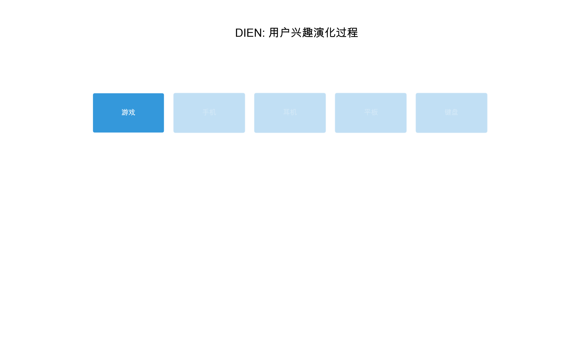
Deep Interest Evolution Network (DIEN)

Motivation

DIN treats all historical behaviors as independent, ignoring the temporal evolution of user interests. DIEN addresses this by modeling how interests evolve over time using a two-layer structure: 1. Interest Extractor Layer: Extracts interests from behavior sequences 2. Interest Evolution Layer: Models how interests evolve

Architecture

Interest Extractor Layer

Uses GRU to extract interest representations from behavior sequences:\[\mathbf{h}_t = \text{GRU}(\mathbf{e}_{b_t}, \mathbf{h}_{t-1})\]where\(\mathbf{e}_{b_t}\)is the embedding of behavior at time\(t\)and\(\mathbf{h}_t\)is the hidden state representing interest at time\(t\).

Interest Evolution Layer

Models interest evolution using an Auxiliary Loss to help the GRU learn meaningful interest representations:

1. Auxiliary Loss: For each time step, predict the next behavior using the current interest representation:\[\mathcal{L}_{aux} = -\frac{1}{N} \sum_{i=1}^{N} \sum_{t=1}^{T} \log \sigma(\mathbf{h}_t^T \mathbf{e}_{b_{t+1 }}^+) + \log(1 - \sigma(\mathbf{h}_t^T \mathbf{e}_{b_{t+1 }}^-))\]where\(\mathbf{e}_{b_{t+1 }}^+\)is the embedding of the actual next behavior and\(\mathbf{e}_{b_{t+1 }}^-\)is a negative sample.

2. Attention-based GRU: Uses attention mechanism to focus on relevant historical interests:\[\alpha_t = \text{Attention}(\mathbf{h}_t, \mathbf{e}_i)\] \[\mathbf{h}_t' = \text{GRU}(\mathbf{h}_t, \mathbf{h}_{t-1}', \alpha_t)\]The final user representation is:\[\mathbf{v}_u = \sum_{t=1}^{T} \alpha_t \mathbf{h}_t'\]

Implementation Example

class InterestExtractorLayer(nn.Module):
    """Extracts interests from behavior sequences using GRU"""
    
    def __init__(self, embedding_dim, hidden_dim=64):
        super(InterestExtractorLayer, self).__init__()
        self.gru = nn.GRU(
            embedding_dim, hidden_dim, batch_first=True, bidirectional=False
        )
        self.hidden_dim = hidden_dim
        
    def forward(self, behavior_sequence):
        """
        Args:
            behavior_sequence: [batch_size, seq_len, embedding_dim]
        Returns:
            interest_sequence: [batch_size, seq_len, hidden_dim]
        """
        interest_sequence, _ = self.gru(behavior_sequence)
        return interest_sequence


class AttentionBasedGRU(nn.Module):
    """Attention-based GRU for interest evolution"""
    
    def __init__(self, hidden_dim):
        super(AttentionBasedGRU, self).__init__()
        self.gru_cell = nn.GRUCell(hidden_dim, hidden_dim)
        self.attention = nn.Linear(hidden_dim * 2, 1)
        
    def forward(self, interest_sequence, candidate_embedding):
        """
        Args:
            interest_sequence: [batch_size, seq_len, hidden_dim]
            candidate_embedding: [batch_size, embedding_dim]
        Returns:
            evolved_interests: [batch_size, seq_len, hidden_dim]
            attention_weights: [batch_size, seq_len]
        """
        batch_size, seq_len, hidden_dim = interest_sequence.shape
        
        # Compute attention weights
        candidate_expanded = candidate_embedding.unsqueeze(1).expand(
            batch_size, seq_len, hidden_dim
        )
        concat_features = torch.cat(
            [interest_sequence, candidate_expanded], dim=-1
        )
        attention_scores = self.attention(concat_features).squeeze(-1)
        attention_weights = F.softmax(attention_scores, dim=1)
        
        # Evolve interests with attention
        evolved_interests = []
        h = torch.zeros(batch_size, hidden_dim).to(interest_sequence.device)
        
        for t in range(seq_len):
            # Combine current interest with attention
            attended_interest = attention_weights[:, t:t+1].unsqueeze(-1) * interest_sequence[:, t, :]
            h = self.gru_cell(attended_interest.squeeze(1), h)
            evolved_interests.append(h)
        
        evolved_interests = torch.stack(evolved_interests, dim=1)
        return evolved_interests, attention_weights


class DIEN(nn.Module):
    """Deep Interest Evolution Network"""
    
    def __init__(
        self,
        item_embedding_dim=64,
        user_feature_dim=32,
        context_feature_dim=16,
        hidden_dims=[200, 80],
        dropout=0.5
    ):
        super(DIEN, self).__init__()
        
        self.interest_extractor = InterestExtractorLayer(
            item_embedding_dim, hidden_dim=64
        )
        self.interest_evolution = AttentionBasedGRU(hidden_dim=64)
        
        # MLP layers
        mlp_input_dim = (
            64 +  # evolved user interest
            item_embedding_dim +  # candidate item
            user_feature_dim +
            context_feature_dim
        )
        
        mlp_layers = []
        input_dim = mlp_input_dim
        for hidden_dim in hidden_dims:
            mlp_layers.append(nn.Linear(input_dim, hidden_dim))
            mlp_layers.append(nn.ReLU())
            mlp_layers.append(nn.Dropout(dropout))
            input_dim = hidden_dim
        
        mlp_layers.append(nn.Linear(input_dim, 1))
        mlp_layers.append(nn.Sigmoid())
        
        self.mlp = nn.Sequential(*mlp_layers)
        
    def forward(
        self,
        user_features,
        behavior_sequence,
        candidate_item,
        context_features
    ):
        """
        Args:
            user_features: [batch_size, user_feature_dim]
            behavior_sequence: [batch_size, seq_len, item_embedding_dim]
            candidate_item: [batch_size, item_embedding_dim]
            context_features: [batch_size, context_feature_dim]
        Returns:
            ctr: [batch_size, 1]
            interest_sequence: [batch_size, seq_len, hidden_dim] (for auxiliary loss)
        """
        # Extract interests
        interest_sequence = self.interest_extractor(behavior_sequence)
        
        # Evolve interests
        evolved_interests, attention_weights = self.interest_evolution(
            interest_sequence, candidate_item
        )
        
        # Use the last evolved interest
        final_user_interest = evolved_interests[:, -1, :]
        
        # Concatenate features
        concat_features = torch.cat([
            final_user_interest,
            candidate_item,
            user_features,
            context_features
        ], dim=1)
        
        # Predict CTR
        ctr = self.mlp(concat_features)
        
        return ctr, interest_sequence

Auxiliary Loss Implementation

class DIENWithAuxiliaryLoss(nn.Module):
    """DIEN with auxiliary loss for training"""
    
    def __init__(self, dien_model, item_embedding_table):
        super(DIENWithAuxiliaryLoss, self).__init__()
        self.dien_model = dien_model
        self.item_embedding_table = item_embedding_table
        
    def compute_auxiliary_loss(self, interest_sequence, next_behaviors):
        """
        Compute auxiliary loss for interest extraction
        
        Args:
            interest_sequence: [batch_size, seq_len-1, hidden_dim]
            next_behaviors: [batch_size, seq_len-1] (item indices)
        Returns:
            auxiliary_loss: scalar
        """
        batch_size, seq_len, hidden_dim = interest_sequence.shape
        
        # Get embeddings of next behaviors
        next_embeddings = self.item_embedding_table(next_behaviors)
        
        # Positive scores: interest predicts next behavior
        positive_scores = torch.sum(
            interest_sequence * next_embeddings, dim=-1
        )  # [batch_size, seq_len-1]
        
        # Negative sampling: random items
        negative_indices = torch.randint(
            0, self.item_embedding_table.num_embeddings,
            (batch_size, seq_len)
        ).to(next_behaviors.device)
        negative_embeddings = self.item_embedding_table(negative_indices)
        
        negative_scores = torch.sum(
            interest_sequence * negative_embeddings, dim=-1
        )
        
        # Binary cross-entropy loss
        positive_loss = F.logsigmoid(positive_scores)
        negative_loss = F.logsigmoid(-negative_scores)
        
        auxiliary_loss = -(positive_loss + negative_loss).mean()
        
        return auxiliary_loss
    
    def forward(
        self,
        user_features,
        behavior_sequence,
        candidate_item,
        context_features,
        next_behaviors=None
    ):
        ctr, interest_sequence = self.dien_model(
            user_features, behavior_sequence, candidate_item, context_features
        )
        
        auxiliary_loss = None
        if next_behaviors is not None and self.training:
            # Use interest sequence except last step
            auxiliary_loss = self.compute_auxiliary_loss(
                interest_sequence[:, :-1, :],
                behavior_sequence[:, 1:, :]  # Next behaviors
            )
        
        return ctr, auxiliary_loss

Deep Session Interest Network (DSIN)

Motivation

User behaviors often occur in sessions — short periods of focused activity. DSIN models session-level patterns by: 1. Splitting behavior sequences into sessions 2. Extracting session-level interests 3. Modeling session evolution 4. Using self-attention within sessions

Architecture

Session Division

Split user behavior sequence into sessions based on time gaps:\[\mathbf{B}_u = [\mathbf{S}_1, \mathbf{S}_2, \dots, \mathbf{S}_K]\]where each session\(\mathbf{S}_k = [b_{k,1}, b_{k,2}, \dots, b_{k,|S_k|}]\)contains behaviors within a time window.

Session Interest Extractor

Uses self-attention within each session to extract session-level interests:\[\text{Attention}(\mathbf{Q}, \mathbf{K}, \mathbf{V}) = \text{softmax}\left(\frac{\mathbf{Q}\mathbf{K}^T}{\sqrt{d }}\right)\mathbf{V}\]where\(\mathbf{Q} = \mathbf{K} = \mathbf{V} = \mathbf{S}_k\)(self-attention).

The session interest is:\[\mathbf{s}_k = \text{Attention}(\mathbf{S}_k, \mathbf{S}_k, \mathbf{S}_k)\]

Bias Encoding

Adds positional and session bias to capture temporal patterns:\[\mathbf{S}_k' = \mathbf{S}_k + \mathbf{B}_{pos} + \mathbf{B}_{session}\]

Session Interest Interacting Layer

Models how session interests evolve using Bi-LSTM:\[\overrightarrow{\mathbf{h }}_k = \text{LSTM}(\mathbf{s}_k, \overrightarrow{\mathbf{h }}_{k-1})\] \[\overleftarrow{\mathbf{h }}_k = \text{LSTM}(\mathbf{s}_k, \overleftarrow{\mathbf{h }}_{k+1})\] \[\mathbf{h}_k = [\overrightarrow{\mathbf{h }}_k; \overleftarrow{\mathbf{h }}_k]\]

Session Interest Activating Layer

Uses target attention to weight session interests:\[\alpha_k = \text{Attention}(\mathbf{h}_k, \mathbf{e}_i)\] \[\mathbf{v}_u = \sum_{k=1}^{K} \alpha_k \mathbf{h}_k\]

Implementation Example

class SessionInterestExtractor(nn.Module):
    """Extracts session-level interests using self-attention"""
    
    def __init__(self, embedding_dim, num_heads=4):
        super(SessionInterestExtractor, self).__init__()
        self.embedding_dim = embedding_dim
        self.num_heads = num_heads
        self.head_dim = embedding_dim // num_heads
        
        self.query = nn.Linear(embedding_dim, embedding_dim)
        self.key = nn.Linear(embedding_dim, embedding_dim)
        self.value = nn.Linear(embedding_dim, embedding_dim)
        self.output = nn.Linear(embedding_dim, embedding_dim)
        
    def forward(self, session_behaviors):
        """
        Args:
            session_behaviors: [batch_size, session_len, embedding_dim]
        Returns:
            session_interest: [batch_size, embedding_dim]
        """
        batch_size, session_len, emb_dim = session_behaviors.shape
        
        Q = self.query(session_behaviors)
        K = self.key(session_behaviors)
        V = self.value(session_behaviors)
        
        # Multi-head attention
        Q = Q.view(batch_size, session_len, self.num_heads, self.head_dim).transpose(1, 2)
        K = K.view(batch_size, session_len, self.num_heads, self.head_dim).transpose(1, 2)
        V = V.view(batch_size, session_len, self.num_heads, self.head_dim).transpose(1, 2)
        
        # Scaled dot-product attention
        scores = torch.matmul(Q, K.transpose(-2, -1)) / math.sqrt(self.head_dim)
        attention_weights = F.softmax(scores, dim=-1)
        attended = torch.matmul(attention_weights, V)
        
        # Concatenate heads
        attended = attended.transpose(1, 2).contiguous().view(
            batch_size, session_len, emb_dim
        )
        
        output = self.output(attended)
        
        # Average pooling to get session interest
        session_interest = output.mean(dim=1)
        
        return session_interest


class BiasEncoding(nn.Module):
    """Bias encoding for sessions"""
    
    def __init__(self, max_session_len, max_sessions, embedding_dim):
        super(BiasEncoding, self).__init__()
        self.pos_bias = nn.Parameter(
            torch.randn(max_session_len, embedding_dim)
        )
        self.session_bias = nn.Parameter(
            torch.randn(max_sessions, embedding_dim)
        )
        
    def forward(self, session_behaviors, session_idx):
        """
        Args:
            session_behaviors: [batch_size, session_len, embedding_dim]
            session_idx: [batch_size] (which session number)
        Returns:
            biased_behaviors: [batch_size, session_len, embedding_dim]
        """
        batch_size, session_len, emb_dim = session_behaviors.shape
        
        # Position bias
        pos_bias = self.pos_bias[:session_len, :].unsqueeze(0)
        
        # Session bias
        session_bias = self.session_bias[session_idx].unsqueeze(1)
        
        biased_behaviors = session_behaviors + pos_bias + session_bias
        
        return biased_behaviors


class SessionInterestInteractingLayer(nn.Module):
    """Models session interest evolution using Bi-LSTM"""
    
    def __init__(self, embedding_dim, hidden_dim=64):
        super(SessionInterestInteractingLayer, self).__init__()
        self.bi_lstm = nn.LSTM(
            embedding_dim, hidden_dim, batch_first=True, bidirectional=True
        )
        self.hidden_dim = hidden_dim
        
    def forward(self, session_interests):
        """
        Args:
            session_interests: [batch_size, num_sessions, embedding_dim]
        Returns:
            evolved_interests: [batch_size, num_sessions, hidden_dim * 2]
        """
        evolved_interests, _ = self.bi_lstm(session_interests)
        return evolved_interests


class DSIN(nn.Module):
    """Deep Session Interest Network"""
    
    def __init__(
        self,
        item_embedding_dim=64,
        user_feature_dim=32,
        context_feature_dim=16,
        hidden_dims=[200, 80],
        max_sessions=10,
        max_session_len=20,
        dropout=0.5
    ):
        super(DSIN, self).__init__()
        
        self.session_extractor = SessionInterestExtractor(
            item_embedding_dim, num_heads=4
        )
        self.bias_encoding = BiasEncoding(
            max_session_len, max_sessions, item_embedding_dim
        )
        self.session_interacting = SessionInterestInteractingLayer(
            item_embedding_dim, hidden_dim=64
        )
        
        # Target attention for session interests
        self.target_attention = nn.Linear(item_embedding_dim + 64 * 2, 1)
        
        # MLP layers
        mlp_input_dim = (
            64 * 2 +  # activated session interests
            item_embedding_dim +  # candidate item
            user_feature_dim +
            context_feature_dim
        )
        
        mlp_layers = []
        input_dim = mlp_input_dim
        for hidden_dim in hidden_dims:
            mlp_layers.append(nn.Linear(input_dim, hidden_dim))
            mlp_layers.append(nn.ReLU())
            mlp_layers.append(nn.Dropout(dropout))
            input_dim = hidden_dim
        
        mlp_layers.append(nn.Linear(input_dim, 1))
        mlp_layers.append(nn.Sigmoid())
        
        self.mlp = nn.Sequential(*mlp_layers)
        
    def forward(
        self,
        user_features,
        sessions,  # List of sessions, each [batch_size, session_len, embedding_dim]
        candidate_item,
        context_features,
        session_indices=None
    ):
        """
        Args:
            user_features: [batch_size, user_feature_dim]
            sessions: List of K sessions, each [batch_size, session_len, embedding_dim]
            candidate_item: [batch_size, item_embedding_dim]
            context_features: [batch_size, context_feature_dim]
            session_indices: [batch_size, K] (session numbers for bias encoding)
        Returns:
            ctr: [batch_size, 1]
            attention_weights: [batch_size, K]
        """
        batch_size = candidate_item.shape[0]
        num_sessions = len(sessions)
        
        # Extract session interests
        session_interests = []
        for k, session in enumerate(sessions):
            if session_indices is not None:
                session = self.bias_encoding(
                    session, session_indices[:, k]
                )
            session_interest = self.session_extractor(session)
            session_interests.append(session_interest)
        
        session_interests = torch.stack(session_interests, dim=1)
        
        # Model session evolution
        evolved_interests = self.session_interacting(session_interests)
        
        # Target attention
        candidate_expanded = candidate_item.unsqueeze(1).expand(
            batch_size, num_sessions, -1
        )
        concat_features = torch.cat(
            [evolved_interests, candidate_expanded], dim=-1
        )
        attention_scores = self.target_attention(concat_features).squeeze(-1)
        attention_weights = F.softmax(attention_scores, dim=1)
        
        # Weighted sum
        activated_interests = torch.sum(
            attention_weights.unsqueeze(-1) * evolved_interests,
            dim=1
        )
        
        # Concatenate features
        concat_features = torch.cat([
            activated_interests,
            candidate_item,
            user_features,
            context_features
        ], dim=1)
        
        # Predict CTR
        ctr = self.mlp(concat_features)
        
        return ctr, attention_weights

Attention Variants

Multi-Head Attention

Multi-head attention allows the model to attend to different aspects simultaneously:\[\text{MultiHead}(\mathbf{Q}, \mathbf{K}, \mathbf{V}) = \text{Concat}(\text{head}_1, \dots, \text{head}_h)\mathbf{W}^O\]where each head is:\[\text{head}_i = \text{Attention}(\mathbf{Q}\mathbf{W}_i^Q, \mathbf{K}\mathbf{W}_i^K, \mathbf{V}\mathbf{W}_i^V)\]

Implementation

class MultiHeadAttention(nn.Module):
    """Multi-head attention mechanism"""
    
    def __init__(self, embedding_dim, num_heads=8):
        super(MultiHeadAttention, self).__init__()
        assert embedding_dim % num_heads == 0
        
        self.embedding_dim = embedding_dim
        self.num_heads = num_heads
        self.head_dim = embedding_dim // num_heads
        
        self.query = nn.Linear(embedding_dim, embedding_dim)
        self.key = nn.Linear(embedding_dim, embedding_dim)
        self.value = nn.Linear(embedding_dim, embedding_dim)
        self.output = nn.Linear(embedding_dim, embedding_dim)
        
    def forward(self, query, key, value, mask=None):
        """
        Args:
            query: [batch_size, seq_len_q, embedding_dim]
            key: [batch_size, seq_len_k, embedding_dim]
            value: [batch_size, seq_len_v, embedding_dim]
            mask: [batch_size, seq_len_q, seq_len_k] (optional)
        Returns:
            output: [batch_size, seq_len_q, embedding_dim]
            attention_weights: [batch_size, num_heads, seq_len_q, seq_len_k]
        """
        batch_size = query.shape[0]
        
        Q = self.query(query)
        K = self.key(key)
        V = self.value(value)
        
        # Reshape for multi-head
        Q = Q.view(batch_size, -1, self.num_heads, self.head_dim).transpose(1, 2)
        K = K.view(batch_size, -1, self.num_heads, self.head_dim).transpose(1, 2)
        V = V.view(batch_size, -1, self.num_heads, self.head_dim).transpose(1, 2)
        
        # Scaled dot-product attention
        scores = torch.matmul(Q, K.transpose(-2, -1)) / math.sqrt(self.head_dim)
        
        if mask is not None:
            scores = scores.masked_fill(mask == 0, -1e9)
        
        attention_weights = F.softmax(scores, dim=-1)
        attended = torch.matmul(attention_weights, V)
        
        # Concatenate heads
        attended = attended.transpose(1, 2).contiguous().view(
            batch_size, -1, self.embedding_dim
        )
        
        output = self.output(attended)
        
        return output, attention_weights

Self-Attention

Self-attention uses the same sequence as query, key, and value:\[\text{SelfAttention}(\mathbf{X}) = \text{Attention}(\mathbf{X}, \mathbf{X}, \mathbf{X})\]This captures relationships within the sequence itself.

Co-Attention

Co-attention models interactions between two sequences (e.g., user behaviors and item features):\[\mathbf{A} = \text{softmax}(\mathbf{X}_1 \mathbf{W}_1 (\mathbf{X}_2 \mathbf{W}_2)^T)\] \[\mathbf{X}_1' = \mathbf{A} \mathbf{X}_2\] \[\mathbf{X}_2' = \mathbf{A}^T \mathbf{X}_1\]

Implementation

class CoAttention(nn.Module):
    """Co-attention between two sequences"""
    
    def __init__(self, embedding_dim1, embedding_dim2, hidden_dim=64):
        super(CoAttention, self).__init__()
        self.linear1 = nn.Linear(embedding_dim1, hidden_dim)
        self.linear2 = nn.Linear(embedding_dim2, hidden_dim)
        
    def forward(self, seq1, seq2):
        """
        Args:
            seq1: [batch_size, len1, embedding_dim1]
            seq2: [batch_size, len2, embedding_dim2]
        Returns:
            attended_seq1: [batch_size, len1, embedding_dim2]
            attended_seq2: [batch_size, len2, embedding_dim1]
        """
        # Project to same dimension
        proj1 = self.linear1(seq1)  # [batch_size, len1, hidden_dim]
        proj2 = self.linear2(seq2)  # [batch_size, len2, hidden_dim]
        
        # Attention matrix
        attention_matrix = torch.matmul(proj1, proj2.transpose(-2, -1))
        attention_matrix = F.softmax(attention_matrix, dim=-1)
        
        # Attend seq2 to seq1
        attended_seq1 = torch.matmul(attention_matrix, seq2)
        
        # Attend seq1 to seq2
        attention_matrix_T = attention_matrix.transpose(-2, -1)
        attended_seq2 = torch.matmul(attention_matrix_T, seq1)
        
        return attended_seq1, attended_seq2

Bilinear Attention

Bilinear attention uses a learned bilinear transformation:\[\text{score}(\mathbf{q}, \mathbf{k}) = \mathbf{q}^T \mathbf{W} \mathbf{k}\]

Implementation

class BilinearAttention(nn.Module):
    """Bilinear attention mechanism"""
    
    def __init__(self, embedding_dim):
        super(BilinearAttention, self).__init__()
        self.bilinear = nn.Bilinear(embedding_dim, embedding_dim, 1)
        
    def forward(self, query, keys):
        """
        Args:
            query: [batch_size, embedding_dim]
            keys: [batch_size, seq_len, embedding_dim]
        Returns:
            attended: [batch_size, embedding_dim]
            attention_weights: [batch_size, seq_len]
        """
        batch_size, seq_len, emb_dim = keys.shape
        
        # Expand query
        query_expanded = query.unsqueeze(1).expand(batch_size, seq_len, emb_dim)
        
        # Compute scores
        scores = self.bilinear(query_expanded, keys).squeeze(-1)
        attention_weights = F.softmax(scores, dim=1)
        
        # Weighted sum
        attended = torch.sum(
            attention_weights.unsqueeze(-1) * keys,
            dim=1
        )
        
        return attended, attention_weights

Alibaba Production Practices

Data Pipeline

Feature Engineering

1. User Features:
   • Demographics: age, gender, city, occupation
   • Behavior statistics: average session length, click-through rate
   • Temporal features: hour of day, day of week, is_weekend
2. Item Features:
   • Categorical: category, brand, shop_id
   • Numerical: price, sales_count, rating
   • Text: title, description (embedded)
3. Behavior Features:
   • Clicked items: last N items
   • Purchased items: last N purchases
   • Viewed categories: category sequence
4. Context Features:
   • Device: mobile, desktop, tablet
   • Platform: iOS, Android, Web
   • Time: timestamp, time since last visit

Feature Storage

• Hive tables: Historical features, user profiles
• Redis: Real-time features, hot items
• Feature stores: Online/offline feature consistency

Model Serving

Online Serving Architecture

User Request → Feature Service → Model Service → Ranking Service → Response
                ↓                  ↓              ↓
            Feature Cache      Model Cache    Result Cache

Optimization Techniques

1. Model Quantization: Reduce model size by 4x with minimal accuracy loss
2. Feature Caching: Cache frequently accessed features
3. Batch Prediction: Process multiple requests together
4. Model Parallelism: Distribute large models across machines

A/B Testing

• Traffic splitting: 1% for new model, 99% for baseline
• Metrics: CTR, CVR, GMV (Gross Merchandise Value)
• Statistical significance testing

Training Optimization

Distributed Training

import torch.distributed as dist
from torch.nn.parallel import DistributedDataParallel

def setup_distributed():
    dist.init_process_group(backend='nccl')
    torch.cuda.set_device(int(os.environ['LOCAL_RANK']))

def train_distributed(model, train_loader, optimizer):
    model = DistributedDataParallel(model)
    
    for epoch in range(num_epochs):
        for batch in train_loader:
            optimizer.zero_grad()
            loss = model(batch)
            loss.backward()
            optimizer.step()

Mixed Precision Training

from torch.cuda.amp import autocast, GradScaler

scaler = GradScaler()

for batch in train_loader:
    optimizer.zero_grad()
    
    with autocast():
        loss = model(batch)
    
    scaler.scale(loss).backward()
    scaler.step(optimizer)
    scaler.update()

Gradient Accumulation

accumulation_steps = 4

for i, batch in enumerate(train_loader):
    loss = model(batch) / accumulation_steps
    loss.backward()
    
    if (i + 1) % accumulation_steps == 0:
        optimizer.step()
        optimizer.zero_grad()

Training Techniques

Dice Activation Function

Dice is an adaptive activation function that performs better than ReLU/PReLU:\[\text{Dice}(x) = x \cdot \sigma(\alpha(x - \bar{x}))\]where\(\bar{x}\)is the mean of\(x\)in the mini-batch and\(\alpha\)is a learnable parameter.

Implementation

class Dice(nn.Module):
    """Dice activation function"""
    
    def __init__(self, embedding_dim):
        super(Dice, self).__init__()
        self.alpha = nn.Parameter(torch.zeros(embedding_dim))
        self.bn = nn.BatchNorm1d(embedding_dim)
        
    def forward(self, x):
        x_norm = self.bn(x)
        p = torch.sigmoid(self.alpha * x_norm)
        return x * p

Label Smoothing

Label smoothing prevents overconfidence:\[y_{smooth} = (1 - \epsilon) \cdot y + \epsilon / K\]where\(\epsilon\)is the smoothing factor and\(K\)is the number of classes.

Focal Loss

Focal loss addresses class imbalance:\[\text{FL}(p_t) = -\alpha_t (1 - p_t)^{\gamma} \log(p_t)\]where\(\alpha_t\)balances class importance and\(\gamma\)focuses on hard examples.

Implementation

class FocalLoss(nn.Module):
    """Focal loss for imbalanced classification"""
    
    def __init__(self, alpha=1.0, gamma=2.0):
        super(FocalLoss, self).__init__()
        self.alpha = alpha
        self.gamma = gamma
        
    def forward(self, predictions, targets):
        bce_loss = F.binary_cross_entropy(
            predictions, targets, reduction='none'
        )
        pt = torch.exp(-bce_loss)
        focal_loss = self.alpha * (1 - pt) ** self.gamma * bce_loss
        return focal_loss.mean()

Negative Sampling

For large item spaces, use negative sampling:

def negative_sampling(positive_items, num_negatives, item_pool):
    """
    Sample negative items
    
    Args:
        positive_items: [batch_size] (positive item indices)
        num_negatives: number of negatives per positive
        item_pool: all possible items
    Returns:
        negative_items: [batch_size, num_negatives]
    """
    batch_size = positive_items.shape[0]
    negative_items = []
    
    for i in range(batch_size):
        pos_item = positive_items[i].item()
        # Sample items that are not the positive
        candidates = item_pool[item_pool != pos_item]
        negatives = torch.randint(
            0, len(candidates), (num_negatives,)
        )
        negative_items.append(candidates[negatives])
    
    return torch.stack(negative_items)

Complete Training Example

import torch
import torch.nn as nn
import torch.optim as optim
from torch.utils.data import Dataset, DataLoader
import numpy as np

class RecommendationDataset(Dataset):
    """Dataset for recommendation training"""
    
    def __init__(self, user_features, behavior_sequences, 
                 candidate_items, context_features, labels):
        self.user_features = torch.FloatTensor(user_features)
        self.behavior_sequences = torch.FloatTensor(behavior_sequences)
        self.candidate_items = torch.FloatTensor(candidate_items)
        self.context_features = torch.FloatTensor(context_features)
        self.labels = torch.FloatTensor(labels)
        
    def __len__(self):
        return len(self.labels)
    
    def __getitem__(self, idx):
        return {
            'user_features': self.user_features[idx],
            'behavior_sequence': self.behavior_sequences[idx],
            'candidate_item': self.candidate_items[idx],
            'context_features': self.context_features[idx],
            'label': self.labels[idx]
        }

def train_din(model, train_loader, val_loader, num_epochs=10, lr=0.001):
    """Complete training loop for DIN"""
    
    device = torch.device('cuda' if torch.cuda.is_available() else 'cpu')
    model = model.to(device)
    
    criterion = nn.BCELoss()
    optimizer = optim.Adam(model.parameters(), lr=lr)
    scheduler = optim.lr_scheduler.ReduceLROnPlateau(
        optimizer, mode='min', factor=0.5, patience=3
    )
    
    best_val_loss = float('inf')
    
    for epoch in range(num_epochs):
        # Training
        model.train()
        train_loss = 0.0
        
        for batch in train_loader:
            user_features = batch['user_features'].to(device)
            behavior_sequence = batch['behavior_sequence'].to(device)
            candidate_item = batch['candidate_item'].to(device)
            context_features = batch['context_features'].to(device)
            labels = batch['label'].to(device)
            
            optimizer.zero_grad()
            
            predictions, attention_weights = model(
                user_features, behavior_sequence, 
                candidate_item, context_features
            )
            
            loss = criterion(predictions.squeeze(), labels)
            loss.backward()
            
            # Gradient clipping
            torch.nn.utils.clip_grad_norm_(model.parameters(), max_norm=1.0)
            
            optimizer.step()
            
            train_loss += loss.item()
        
        train_loss /= len(train_loader)
        
        # Validation
        model.eval()
        val_loss = 0.0
        val_auc = 0.0
        
        with torch.no_grad():
            for batch in val_loader:
                user_features = batch['user_features'].to(device)
                behavior_sequence = batch['behavior_sequence'].to(device)
                candidate_item = batch['candidate_item'].to(device)
                context_features = batch['context_features'].to(device)
                labels = batch['label'].to(device)
                
                predictions, _ = model(
                    user_features, behavior_sequence,
                    candidate_item, context_features
                )
                
                loss = criterion(predictions.squeeze(), labels)
                val_loss += loss.item()
                
                # Compute AUC (simplified)
                predictions_np = predictions.cpu().numpy()
                labels_np = labels.cpu().numpy()
                val_auc += compute_auc(labels_np, predictions_np)
        
        val_loss /= len(val_loader)
        val_auc /= len(val_loader)
        
        scheduler.step(val_loss)
        
        print(f'Epoch {epoch+1}/{num_epochs}:')
        print(f'  Train Loss: {train_loss:.4f}')
        print(f'  Val Loss: {val_loss:.4f}')
        print(f'  Val AUC: {val_auc:.4f}')
        
        # Save best model
        if val_loss < best_val_loss:
            best_val_loss = val_loss
            torch.save(model.state_dict(), 'best_din_model.pth')
    
    return model

def compute_auc(y_true, y_pred):
    """Compute AUC score"""
    from sklearn.metrics import roc_auc_score
    return roc_auc_score(y_true, y_pred)

Evaluation Metrics

CTR Prediction Metrics

1. AUC (Area Under ROC Curve): Measures ranking quality
2. Log Loss: Measures prediction calibration
3. Precision@K: Precision of top K predictions
4. Recall@K: Recall of top K predictions

Implementation

from sklearn.metrics import roc_auc_score, log_loss, precision_recall_curve

def evaluate_model(model, test_loader, device):
    """Evaluate model on test set"""
    model.eval()
    all_predictions = []
    all_labels = []
    
    with torch.no_grad():
        for batch in test_loader:
            user_features = batch['user_features'].to(device)
            behavior_sequence = batch['behavior_sequence'].to(device)
            candidate_item = batch['candidate_item'].to(device)
            context_features = batch['context_features'].to(device)
            labels = batch['label'].to(device)
            
            predictions, _ = model(
                user_features, behavior_sequence,
                candidate_item, context_features
            )
            
            all_predictions.append(predictions.cpu().numpy())
            all_labels.append(labels.cpu().numpy())
    
    all_predictions = np.concatenate(all_predictions)
    all_labels = np.concatenate(all_labels)
    
    auc = roc_auc_score(all_labels, all_predictions)
    logloss = log_loss(all_labels, all_predictions)
    
    return {
        'AUC': auc,
        'Log Loss': logloss
    }

Q&A Section

Q1: Why does DIN use target attention instead of self-attention?

A: Target attention allows the model to focus on historical behaviors that are relevant to the current candidate item. Self-attention would only capture relationships within the behavior sequence itself, but wouldn't connect behaviors to the candidate. For example, if a user clicked on "laptop" and "phone" in the past, and the candidate is "laptop charger", target attention would give higher weight to the "laptop" click, while self-attention might just learn that "laptop" and "phone" are related (both electronics) but wouldn't connect them to "laptop charger".

Q2: How does DIEN's auxiliary loss help training?

A: The auxiliary loss encourages the GRU to learn meaningful interest representations by predicting the next behavior. This acts as a regularizer: if the interest representation\(\mathbf{h}_t\)can predict what the user will click next, it must have captured useful information about the user's current interest state. Without this loss, the GRU might learn trivial representations that don't capture interest evolution.

Q3: What's the difference between DIN, DIEN, and DSIN?

A: - DIN: Models user interests as a weighted sum of historical behaviors using target attention. Treats behaviors as independent. - DIEN: Models how interests evolve over time using GRU, capturing temporal dependencies in user behavior. - DSIN: Splits behaviors into sessions and models session-level patterns using self-attention within sessions and Bi-LSTM across sessions.

Q4: How do you handle variable-length behavior sequences?

A: Common approaches: 1. Padding: Pad shorter sequences with zeros and use masking to ignore padding in attention 2. Truncation: Keep only the last N behaviors 3. Sampling: Randomly sample N behaviors from the sequence 4. Hierarchical: Use RNN/LSTM to encode variable-length sequences into fixed-length vectors

Implementation with masking:

def create_attention_mask(sequence_lengths, max_len):
    """
    Create attention mask for variable-length sequences
    
    Args:
        sequence_lengths: [batch_size] (actual lengths)
        max_len: maximum sequence length
    Returns:
        mask: [batch_size, max_len] (1 for valid, 0 for padding)
    """
    batch_size = len(sequence_lengths)
    mask = torch.zeros(batch_size, max_len)
    
    for i, length in enumerate(sequence_lengths):
        mask[i, :length] = 1
    
    return mask

# In attention computation
attention_scores = attention_scores.masked_fill(mask == 0, -1e9)

Q5: How does multi-head attention help in recommendation?

A: Multi-head attention allows the model to attend to different aspects simultaneously. For example, one head might focus on item categories (laptop → laptop charger), another on brands (Apple → Apple accessories), another on price ranges (budget items → budget items), and another on temporal patterns (recent clicks → similar recent items). This captures richer relationships than single-head attention.

Q6: What are the computational costs of attention mechanisms?

A: Attention has quadratic complexity\(O(n^2)\)in sequence length: - Time:\(O(n^2 \cdot d)\)where\(n\)is sequence length and\(d\)is embedding dimension - Space:\(O(n^2)\)for attention matrix storage

For long sequences (e.g., 1000+ behaviors), this becomes expensive. Solutions: 1. Truncation: Keep only recent N behaviors 2. Sampling: Sample N behaviors instead of using all 3. Sparse attention: Only attend to a subset of positions 4. Linear attention: Use approximations to reduce complexity

Q7: How do you handle cold-start users with few behaviors?

A: For users with sparse behavior histories: 1. Use side features: Rely more on user profile features (demographics, location) 2. Content-based: Use item features when behavior is insufficient 3. Transfer learning: Use embeddings learned from similar users 4. Default behaviors: Use popular items or category-level behaviors as fallback

Implementation:

def handle_sparse_behavior(behavior_sequence, user_features, min_behaviors=5):
    """
    Handle sparse behavior sequences
    
    Args:
        behavior_sequence: [batch_size, seq_len, embedding_dim]
        user_features: [batch_size, feature_dim]
        min_behaviors: minimum behaviors required
    Returns:
        enhanced_sequence: [batch_size, seq_len, embedding_dim]
    """
    batch_size, seq_len, emb_dim = behavior_sequence.shape
    
    # Count non-zero behaviors (assuming padding is zeros)
    behavior_counts = (behavior_sequence.sum(dim=-1) != 0).sum(dim=1)
    
    # For sparse users, use user features as additional "behavior"
    sparse_mask = behavior_counts < min_behaviors
    
    # Expand user features to match behavior dimension
    user_feature_expanded = user_features.unsqueeze(1).expand(
        batch_size, seq_len, -1
    )
    
    # Concatenate or replace for sparse users
    if sparse_mask.any():
        # Option 1: Concatenate
        enhanced_sequence = torch.cat(
            [behavior_sequence, user_feature_expanded], dim=-1
        )
        # Option 2: Replace padding with user features
        # behavior_sequence[sparse_mask] = user_feature_expanded[sparse_mask]
    
    return enhanced_sequence

Q8: How does DSIN's session division work in practice?

A: Sessions are typically divided based on: 1. Time gaps: If time between behaviors > threshold (e.g., 30 minutes), start new session 2. Category changes: If user switches to different category, start new session 3. Explicit signals: User closes app, starts new search, etc.

Implementation:

def divide_into_sessions(behaviors, timestamps, time_threshold=1800):
    """
    Divide behavior sequence into sessions
    
    Args:
        behaviors: [seq_len, embedding_dim]
        timestamps: [seq_len] (Unix timestamps)
        time_threshold: seconds between behaviors to start new session
    Returns:
        sessions: List of sessions, each [session_len, embedding_dim]
    """
    sessions = []
    current_session = [behaviors[0]]
    
    for i in range(1, len(behaviors)):
        time_gap = timestamps[i] - timestamps[i-1]
        
        if time_gap > time_threshold:
            # Start new session
            sessions.append(torch.stack(current_session))
            current_session = [behaviors[i]]
        else:
            current_session.append(behaviors[i])
    
    # Add last session
    if current_session:
        sessions.append(torch.stack(current_session))
    
    return sessions

Q9: What's the role of bias encoding in DSIN?

A: Bias encoding adds positional and session-level information: 1. Positional bias: Captures that behaviors at different positions in a session have different importance (e.g., first click vs. last click) 2. Session bias: Captures that different sessions have different characteristics (e.g., morning browsing vs. evening shopping)

This helps the model understand temporal patterns beyond just the content of behaviors.

Q10: How do you optimize attention for production serving?

A: Production optimizations:

1. Pre-compute attention: For fixed candidate items, pre-compute attention weights
2. Cache embeddings: Cache item and user embeddings
3. Approximate attention: Use low-rank approximations or locality-sensitive hashing
4. Batch processing: Process multiple requests together
5. Model quantization: Reduce precision (FP32 → FP16 → INT8)

Example with caching:

class CachedAttention(nn.Module):
    """Attention with caching for production"""
    
    def __init__(self, embedding_dim):
        super(CachedAttention, self).__init__()
        self.embedding_dim = embedding_dim
        self.attention_cache = {}
        
    def forward(self, behavior_embeddings, candidate_embedding, use_cache=True):
        # Create cache key from candidate embedding hash
        cache_key = hash(candidate_embedding.cpu().numpy().tobytes())
        
        if use_cache and cache_key in self.attention_cache:
            attention_weights = self.attention_cache[cache_key]
        else:
            # Compute attention
            scores = torch.matmul(
                behavior_embeddings, candidate_embedding.unsqueeze(-1)
            ).squeeze(-1)
            attention_weights = F.softmax(scores, dim=1)
            
            if use_cache:
                self.attention_cache[cache_key] = attention_weights
        
        return attention_weights

Q11: How does attention help with model interpretability?

A: Attention weights provide interpretability: 1. Feature importance: Show which historical behaviors matter most 2. Debugging: Identify why certain recommendations were made 3. Business insights: Understand user interest patterns 4. A/B testing: Compare attention patterns between model versions

Visualization example:

def visualize_attention(attention_weights, behavior_items, candidate_item):
    """
    Visualize attention weights
    
    Args:
        attention_weights: [seq_len] (attention weights)
        behavior_items: List of item names/IDs
        candidate_item: Candidate item name/ID
    """
    import matplotlib.pyplot as plt
    
    # Sort by attention weight
    sorted_indices = torch.argsort(attention_weights, descending=True)
    
    print(f"Candidate Item: {candidate_item}")
    print("\nTop Attended Behaviors:")
    for idx in sorted_indices[:10]:
        print(f"  {behavior_items[idx]}: {attention_weights[idx]:.4f}")
    
    # Plot
    plt.figure(figsize=(10, 6))
    plt.barh(range(len(attention_weights)), attention_weights.numpy())
    plt.yticks(range(len(behavior_items)), behavior_items)
    plt.xlabel('Attention Weight')
    plt.title(f'Attention Weights for Candidate: {candidate_item}')
    plt.tight_layout()
    plt.show()

Q12: What are common pitfalls when implementing attention in recommendation?

A: Common pitfalls:

1. Ignoring padding: Not masking padding tokens leads to incorrect attention
2. Gradient vanishing: Very long sequences cause gradient issues
3. Overfitting: Attention can memorize training patterns
4. Computational cost: Not optimizing for production latency
5. Cold-start: Not handling sparse behavior sequences

Solutions:

# 1. Always use masking
attention_scores = attention_scores.masked_fill(mask == 0, -1e9)

# 2. Gradient clipping
torch.nn.utils.clip_grad_norm_(model.parameters(), max_norm=1.0)

# 3. Regularization
loss = criterion(predictions, labels) + lambda_reg * attention_weights.norm()

# 4. Sequence length limits
max_seq_len = 50  # Truncate long sequences

# 5. Sparse behavior handling
if behavior_count < min_behaviors:
    use_content_features = True

Conclusion

Deep Interest Networks and attention mechanisms have revolutionized recommendation systems by enabling models to focus on relevant historical behaviors. DIN's target attention, DIEN's interest evolution modeling, and DSIN's session-aware architecture each address different aspects of the recommendation problem, leading to significant improvements in CTR prediction and user engagement.

The key insights are: 1. Not all behaviors are equal: Target attention weights behaviors by relevance 2. Interests evolve: Temporal modeling captures changing preferences 3. Sessions matter: Session-level patterns provide additional signal 4. Production matters: Optimizations for scale and latency are crucial

As recommendation systems continue to evolve, attention mechanisms remain a fundamental building block, enabling models to understand user interests at increasingly granular levels while maintaining interpretability and efficiency.