Essence of Linear Algebra (15): Linear Algebra in Machine Learning

If you ask a machine learning engineer "what math do you use most often?", the answer is almost certainly linear algebra. From vector representations of data, to forward propagation in neural networks, to matrix factorization in recommender systems — linear algebra is the "native language" of machine learning. This chapter starts from intuition and dives deep into the linear algebra principles behind these core algorithms.

Vector Representations in Machine Learning

Data as Vectors

The first step in machine learning is converting real-world objects into vectors. A pixel handwritten digit image can be flattened into a 784-dimensional vector; a piece of text can be converted to a vector using word frequency statistics or word embeddings; a user's behavior history can be encoded as a feature vector.

Why do this? Because vectors are the fundamental objects of linear algebra operations. Once data becomes vectors, we can:

• Compute distances (Euclidean distance, cosine distance)
• Form linear combinations (feature weighting)
• Perform projections (dimensionality reduction)
• Apply matrix multiplication (feature transformation)

Geometry of Feature Space

Suppose we have samples, each with features. We organize the data into a matrix:

where is the feature vector of sample . Geometrically, each sample is a point in -dimensional space.

This perspective is crucial: many machine learning tasks are essentially geometric operations in high-dimensional space:

• Classification: Find a hyperplane separating points of different classes
• Clustering: Find natural groupings of points
• Dimensionality reduction: Project high-dimensional points to a lower-dimensional subspace
• Regression: Find a hyperplane as close as possible to all points

Word Embeddings: Vectorizing Semantics

Word2Vec, GloVe, and other embedding methods map words to low-dimensional vector spaces, placing semantically similar words closer together. More remarkably, these vectors can perform "semantic arithmetic":

This shows word embeddings capture some linear structure: the gender difference is encoded as a direction vector .

import numpy as np
from gensim.models import KeyedVectors

# Load pre-trained word vectors
model = KeyedVectors.load_word2vec_format('GoogleNews-vectors-negative300.bin', binary=True)

# Semantic arithmetic
result = model.most_similar(positive=['king', 'woman'], negative=['man'], topn=1)
print(result)  # [('queen', 0.7118)]

# Compute cosine similarity between word vectors
similarity = model.similarity('cat', 'dog')
print(f"Similarity between cat and dog: {similarity:.4f}")

Principal Component Analysis (PCA)

Starting from Intuition: Finding the "Principal Axes" of Data

Imagine paper clips scattered on a table. Looking down from above, you notice they roughly align along a certain direction (because paper clips are elongated). PCA's job is to find this "principal direction."

More formally: PCA seeks the direction of maximum data variance. Why focus on variance? Because directions with large variance contain more information, while directions with small variance may just be noise.

Mathematical Derivation

Assume data is centered (zero mean). We want to find a unit vector that maximizes variance when data is projected onto it:

Denoting the covariance matrix , the problem becomes:

Using Lagrange multipliers:

We get . This is an eigenvalue problem! The optimal is the eigenvector corresponding to the largest eigenvalue of the covariance matrix.

Relationship Between PCA and SVD

In practice, PCA is usually computed not by directly forming the covariance matrix (which can be huge when features are many), but by using SVD. For centered data matrix :

Here, columns of are the principal component directions (eigenvectors of the covariance matrix), and diagonal elements of squared divided by give the corresponding variances (eigenvalues).

import numpy as np
from sklearn.preprocessing import StandardScaler
from sklearn.decomposition import PCA
import matplotlib.pyplot as plt

# Generate simulated data: correlated 2D data
np.random.seed(42)
n_samples = 200
theta = np.pi / 6  # Angle of principal direction with x-axis
X = np.random.randn(n_samples, 2) @ np.array([[2, 0], [0, 0.5]])
rotation = np.array([[np.cos(theta), -np.sin(theta)],
                     [np.sin(theta), np.cos(theta)]])
X = X @ rotation

# Method 1: Using sklearn
pca = PCA(n_components=2)
X_pca = pca.fit_transform(X)
print("Principal component directions:\n", pca.components_)
print("Explained variance ratio:", pca.explained_variance_ratio_)

# Method 2: Manual implementation using SVD
X_centered = X - X.mean(axis=0)
U, S, Vt = np.linalg.svd(X_centered, full_matrices=False)
print("\nPrincipal directions from SVD:\n", Vt)
print("Variance:", S**2 / n_samples)

# Visualization
fig, axes = plt.subplots(1, 2, figsize=(12, 5))

# Original data with principal component directions
axes[0].scatter(X[:, 0], X[:, 1], alpha=0.5)
for i, (comp, var) in enumerate(zip(pca.components_, pca.explained_variance_)):
    axes[0].arrow(0, 0, comp[0]*np.sqrt(var)*2, comp[1]*np.sqrt(var)*2,
                  head_width=0.2, head_length=0.1, fc=['r', 'b'][i], ec=['r', 'b'][i])
axes[0].set_title('Original Data with Principal Directions')
axes[0].set_xlabel('x1')
axes[0].set_ylabel('x2')
axes[0].axis('equal')

# Transformed data
axes[1].scatter(X_pca[:, 0], X_pca[:, 1], alpha=0.5)
axes[1].set_title('Data After PCA')
axes[1].set_xlabel('PC1')
axes[1].set_ylabel('PC2')
axes[1].axis('equal')

plt.tight_layout()
plt.savefig('pca_visualization.png', dpi=150)

Applications of PCA

Data visualization: Project high-dimensional data to 2D or 3D for human inspection. For example, project 784-dimensional MNIST images to 2D to see how different digits distribute.

Dimensionality reduction and compression: Keep the firstprincipal components, discard the rest, achieving data compression. If the first 10 components explain 95% of variance, using 10 dimensions instead of 1000 loses little information.

Denoising: Assume signal lies in major components and noise in minor components. Keeping major components filters out noise.

Feature decorrelation: After PCA, new features are orthogonal (uncorrelated), which helps certain algorithms (like Naive Bayes).

Kernel PCA: Handling Nonlinear Structure

Standard PCA only finds linear structure. If data lies on a curved manifold (like a "Swiss roll"), PCA is helpless.

Kernel PCA's idea: First map data to a high-dimensional feature space , then do PCA in feature space. But we don't need to explicitly compute , only the inner product , which can be computed directly using a kernel function .

from sklearn.decomposition import KernelPCA
from sklearn.datasets import make_moons

# Generate nonlinearly separable data
X, y = make_moons(n_samples=200, noise=0.1, random_state=42)

# Linear PCA
pca = PCA(n_components=2)
X_pca = pca.fit_transform(X)

# Kernel PCA (using RBF kernel)
kpca = KernelPCA(n_components=2, kernel='rbf', gamma=10)
X_kpca = kpca.fit_transform(X)

# Compare results
fig, axes = plt.subplots(1, 3, figsize=(15, 4))
axes[0].scatter(X[:, 0], X[:, 1], c=y, cmap='viridis')
axes[0].set_title('Original Data')
axes[1].scatter(X_pca[:, 0], X_pca[:, 1], c=y, cmap='viridis')
axes[1].set_title('Linear PCA')
axes[2].scatter(X_kpca[:, 0], X_kpca[:, 1], c=y, cmap='viridis')
axes[2].set_title('Kernel PCA (RBF)')
plt.savefig('kernel_pca.png', dpi=150)

Linear Discriminant Analysis (LDA)

Supervised Dimensionality Reduction

PCA is unsupervised — it doesn't know class labels. LDA is supervised: it uses class information to find projection directions that best separate different classes.

Intuitively, LDA seeks a direction where: 1. Class centers are as far apart as possible after projection (large between-class distance) 2. Points within each class are as close together as possible after projection (small within-class variance)

Mathematical Formulation

Let there beclasses, with classhavingsamples, mean, and overall mean.

Within-class scatter matrix (measuring dispersion within each class):

Between-class scatter matrix (measuring dispersion between class centers):

LDA maximizes the generalized Rayleigh quotient:

This is equivalent to solving the generalized eigenvalue problem .

Fisher Discriminant for Binary Classification

For two-class problems, Fisher gave a more direct derivation. Projected between-class distance is , within-class variance is . Fisher's criterion:

The optimal solution is .

from sklearn.discriminant_analysis import LinearDiscriminantAnalysis
from sklearn.datasets import load_iris
import numpy as np
import matplotlib.pyplot as plt

# Load iris dataset
iris = load_iris()
X, y = iris.data, iris.target

# LDA reduction to 2D
lda = LinearDiscriminantAnalysis(n_components=2)
X_lda = lda.fit_transform(X, y)

# PCA reduction to 2D (for comparison)
pca = PCA(n_components=2)
X_pca = pca.fit_transform(X)

# Visual comparison
fig, axes = plt.subplots(1, 2, figsize=(12, 5))

for i, (X_transformed, title) in enumerate([(X_pca, 'PCA'), (X_lda, 'LDA')]):
    for label in np.unique(y):
        axes[i].scatter(X_transformed[y==label, 0], X_transformed[y==label, 1],
                       label=iris.target_names[label], alpha=0.7)
    axes[i].set_title(f'{title} Dimensionality Reduction')
    axes[i].legend()

plt.tight_layout()
plt.savefig('lda_vs_pca.png', dpi=150)

# Print LDA explained variance ratio
print(f"LDA explained variance ratio: {lda.explained_variance_ratio_}")

PCA vs LDA: When to Use Which?

Property	PCA	LDA
Supervision	Unsupervised	Supervised
Objective	Maximize variance	Maximize class separability
Max dimensions
Use cases	Data exploration, compression, denoising	Classification preprocessing
Assumptions	Linear structure	Gaussian within-class, same covariance

An important limitation: LDA can reduce to at mostdimensions (is number of classes). For binary classification, LDA can only reduce to 1D.

Support Vector Machines and Kernel Methods

Linear SVM: Maximum Margin Classifier

Support vector machines seek a hyperplaneseparating two classes with maximum margin.

What is margin? Intuitively, it's the distance from the hyperplane to the nearest data points. The distance from pointto the hyperplane is. For correctly classified points,.

By appropriately scalingand, we can make the nearest points satisfy. Then the margin is.

Optimization Problem

Primal problem:

Using Lagrange multipliers, introduce :

Dual problem (after optimizing over and ):

Notice the dual only involves inner products between data points. This is key to the kernel trick!

The Kernel Trick

If data is linearly inseparable, one approach is mapping data to a higher-dimensional space. For example, for 2D data, map to:A circular boundary in the original space may become linear in the new space.

The problem is: high-dimensional mappings are computationally expensive. The beauty of the kernel trick is that we only need to compute inner products, which can be done directly with a simple function, without explicitly computing.

Common kernel functions:

• Linear kernel:
• Polynomial kernel:
• RBF kernel (Gaussian):
• Sigmoid kernel:

The RBF kernel corresponds to an infinite-dimensional feature space! But computing inner products only takes time.

Kernel Matrix and Positive Definiteness

Given data points, the kernel matrix (Gram matrix) is defined as:

A function is a valid kernel if and only if for any dataset, the kernel matrix is positive semi-definite (all eigenvalues ). This is called the Mercer condition.

Intuitively, theelement of the kernel matrix measures "similarity" between samplesand. Positive semi-definiteness ensures this similarity measure is self-consistent.

from sklearn.svm import SVC
from sklearn.datasets import make_circles
import numpy as np
import matplotlib.pyplot as plt

# Generate ring data (linearly inseparable)
X, y = make_circles(n_samples=200, noise=0.1, factor=0.3, random_state=42)

# Linear SVM
svm_linear = SVC(kernel='linear')
svm_linear.fit(X, y)

# RBF kernel SVM
svm_rbf = SVC(kernel='rbf', gamma=2)
svm_rbf.fit(X, y)

# Visualize decision boundaries
def plot_decision_boundary(ax, clf, X, y, title):
    xx, yy = np.meshgrid(np.linspace(X[:, 0].min()-0.5, X[:, 0].max()+0.5, 200),
                         np.linspace(X[:, 1].min()-0.5, X[:, 1].max()+0.5, 200))
    Z = clf.predict(np.c_[xx.ravel(), yy.ravel()]).reshape(xx.shape)
    ax.contourf(xx, yy, Z, alpha=0.3, cmap='coolwarm')
    ax.scatter(X[:, 0], X[:, 1], c=y, cmap='coolwarm', edgecolors='black')
    ax.set_title(title)
    # Mark support vectors
    ax.scatter(clf.support_vectors_[:, 0], clf.support_vectors_[:, 1],
               s=100, facecolors='none', edgecolors='green', linewidths=2)

fig, axes = plt.subplots(1, 2, figsize=(12, 5))
plot_decision_boundary(axes[0], svm_linear, X, y, 'Linear SVM')
plot_decision_boundary(axes[1], svm_rbf, X, y, 'RBF Kernel SVM')
plt.tight_layout()
plt.savefig('svm_kernels.png', dpi=150)

print(f"Linear SVM accuracy: {svm_linear.score(X, y):.2f}")
print(f"RBF kernel SVM accuracy: {svm_rbf.score(X, y):.2f}")
print(f"Number of support vectors: {len(svm_rbf.support_vectors_)}")

Matrix Factorization and Recommender Systems

The Netflix Problem

A classic recommender system problem: There is a user-movie rating matrix(users,movies), but most elements are missing (users can't have watched all movies). The goal is to predict missing ratings and recommend movies users might like.

Low-Rank Assumption

Core assumption: User preferences and movie characteristics can be described by a small number of "latent factors." For example, factors might correspond to "action level," "romance level," "star presence," etc.

Mathematically, assume, where(user factor matrix),(item factor matrix),.

User's predicted rating for movieis.

Optimization Objective

Optimize only on observed ratings (with regularization):

where is the set of observed positions and is the regularization coefficient.

Alternating Least Squares (ALS)

This problem is non-convex jointly in, but convex (quadratic programming) when fixing one and optimizing the other. ALS alternates:

1. Fix, update: Eachindependently solves a ridge regression
2. Fix, update: Eachindependently solves a ridge regression
3. Repeat until convergence

import numpy as np
from scipy.sparse import random as sparse_random
from scipy.sparse.linalg import svds

# Simulate a rating matrix
np.random.seed(42)
n_users, n_items, k = 100, 50, 5

# True low-rank structure
U_true = np.random.randn(n_users, k)
V_true = np.random.randn(n_items, k)
R_true = U_true @ V_true.T

# Observe only 20% of ratings, add noise
mask = np.random.rand(n_users, n_items) < 0.2
R_observed = np.where(mask, R_true + 0.1 * np.random.randn(n_users, n_items), 0)

# ALS algorithm
def als(R_observed, mask, k, n_iter=50, lambda_reg=0.1):
    n_users, n_items = R_observed.shape
    U = np.random.randn(n_users, k) * 0.1
    V = np.random.randn(n_items, k) * 0.1
    
    for iteration in range(n_iter):
        # Update U
        for i in range(n_users):
            items_rated = np.where(mask[i, :])[0]
            if len(items_rated) > 0:
                V_sub = V[items_rated, :]
                r_sub = R_observed[i, items_rated]
                U[i, :] = np.linalg.solve(V_sub.T @ V_sub + lambda_reg * np.eye(k),
                                          V_sub.T @ r_sub)
        
        # Update V
        for j in range(n_items):
            users_rated = np.where(mask[:, j])[0]
            if len(users_rated) > 0:
                U_sub = U[users_rated, :]
                r_sub = R_observed[users_rated, j]
                V[j, :] = np.linalg.solve(U_sub.T @ U_sub + lambda_reg * np.eye(k),
                                          U_sub.T @ r_sub)
        
        # Compute loss
        if iteration % 10 == 0:
            R_pred = U @ V.T
            loss = np.sum((R_observed[mask] - R_pred[mask])**2)
            print(f"Iteration {iteration}, Loss: {loss:.4f}")
    
    return U, V

U_learned, V_learned = als(R_observed, mask, k)

# Predict missing ratings
R_pred = U_learned @ V_learned.T
rmse = np.sqrt(np.mean((R_true[~mask] - R_pred[~mask])**2))
print(f"\nRMSE on unobserved positions: {rmse:.4f}")

Non-negative Matrix Factorization (NMF)

Sometimes we want decomposition results to be non-negative for interpretability. For example, in document-word matrix factorization, non-negative factors can be interpreted as "topics."NMF tends to produce sparse, parts-based representations, unlike SVD's global representations that may have positive and negative values.

from sklearn.decomposition import NMF
from sklearn.datasets import fetch_20newsgroups
from sklearn.feature_extraction.text import TfidfVectorizer

# Load news data
categories = ['rec.sport.baseball', 'sci.med', 'comp.graphics']
newsgroups = fetch_20newsgroups(subset='train', categories=categories)

# TF-IDF vectorization
vectorizer = TfidfVectorizer(max_features=1000, stop_words='english')
X = vectorizer.fit_transform(newsgroups.data)

# NMF decomposition
n_topics = 5
nmf = NMF(n_components=n_topics, random_state=42)
W = nmf.fit_transform(X)  # document-topic matrix
H = nmf.components_  # topic-word matrix

# Show top words for each topic
feature_names = vectorizer.get_feature_names_out()
for topic_idx, topic in enumerate(H):
    top_words = [feature_names[i] for i in topic.argsort()[:-10:-1]]
    print(f"Topic {topic_idx}: {', '.join(top_words)}")

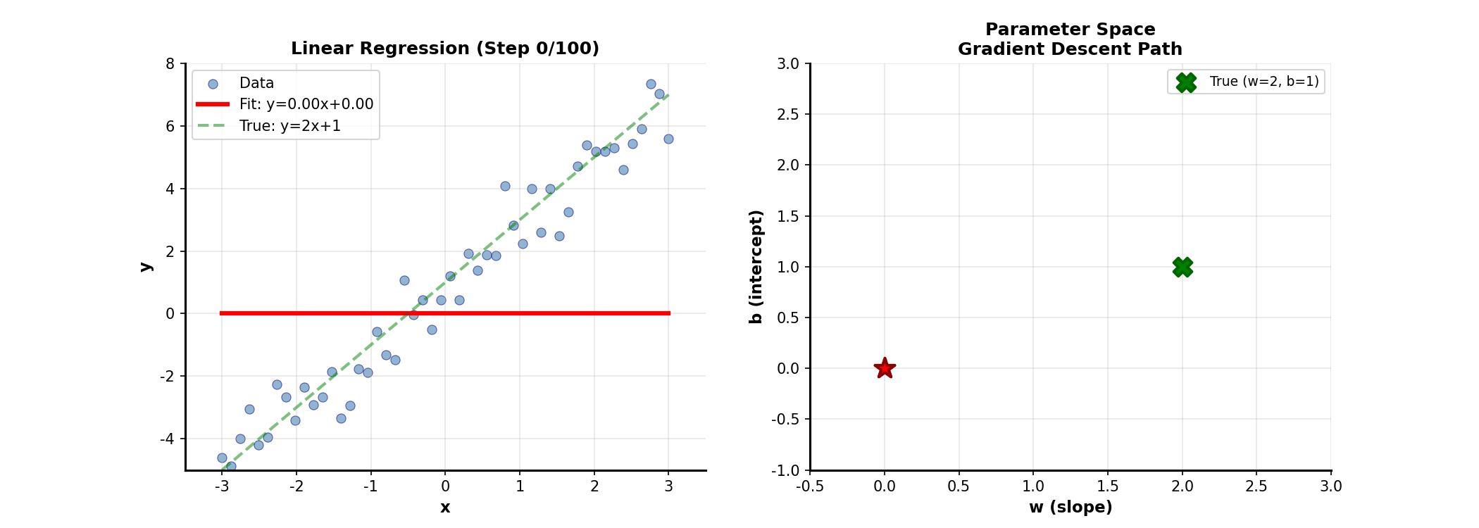
Matrix Form of Linear Regression

From Scalars to Matrices

The familiar simple linear regression generalizes to multiple variables as:

Stacking all samples, in matrix form:

where is the design matrix (including intercept column), is the response vector, is the parameter vector.

Geometric Interpretation of Least Squares

Least squares minimizes residual sum of squares:

Geometrically, is a vector in the column space of . We seek the point in 's column space closest to . The answer: the projection of onto 's column space!

The optimal satisfies that residual is orthogonal to 's column space:

Solving gives the normal equations:

Numerical Stability Issues

Directly computinghas two problems:

1. When(more features than samples),is not invertible
2. When features are highly correlated,is ill-conditioned (large condition number), leading to numerical instability

A better approach uses QR decomposition:, then. Sinceis upper triangular, back-substitution is stable.

Ridge Regression: Solving Ill-conditioning

Ridge regression adds an penalty to the loss:

The solution is:

Adding ensures invertibility and improves the condition number. From an SVD perspective, if , then:

Components corresponding to small singular values are "shrunk," reducing overfitting.

LASSO: Sparse Feature Selection

LASSO uses penalty instead of :

The magic of penalty is that it produces sparse solutions: many will be exactly zero. This performs automatic feature selection.

Why? Geometrically, the constraint region is a "diamond" (hypercube), while loss function level curves are ellipses. They most likely touch at diamond vertices — where some coordinates are zero.

import numpy as np
from sklearn.linear_model import LinearRegression, Ridge, Lasso
from sklearn.preprocessing import StandardScaler
import matplotlib.pyplot as plt

# Generate data: only first 3 features are useful
np.random.seed(42)
n, p = 100, 20
X = np.random.randn(n, p)
beta_true = np.zeros(p)
beta_true[:3] = [3, -2, 1.5]  # Only first 3 features matter
y = X @ beta_true + 0.5 * np.random.randn(n)

# Standardize
scaler = StandardScaler()
X_scaled = scaler.fit_transform(X)

# Ordinary least squares
ols = LinearRegression(fit_intercept=False)
ols.fit(X_scaled, y)

# Ridge regression
ridge = Ridge(alpha=1.0, fit_intercept=False)
ridge.fit(X_scaled, y)

# LASSO
lasso = Lasso(alpha=0.1, fit_intercept=False)
lasso.fit(X_scaled, y)

# Compare coefficients
fig, ax = plt.subplots(figsize=(12, 5))
x_pos = np.arange(p)
width = 0.25

ax.bar(x_pos - width, beta_true, width, label='True coefficients', alpha=0.7)
ax.bar(x_pos, ols.coef_, width, label='OLS', alpha=0.7)
ax.bar(x_pos + width, lasso.coef_, width, label='LASSO', alpha=0.7)
ax.axhline(y=0, color='black', linestyle='-', linewidth=0.5)
ax.set_xlabel('Feature index')
ax.set_ylabel('Coefficient value')
ax.set_title('Comparison of Regression Methods')
ax.legend()
plt.tight_layout()
plt.savefig('regression_comparison.png', dpi=150)

print(f"OLS nonzero coefficients: {np.sum(np.abs(ols.coef_) > 0.01)}")
print(f"LASSO nonzero coefficients: {np.sum(np.abs(lasso.coef_) > 0.01)}")

Linear Layers in Neural Networks

Fully Connected Layers Are Matrix Multiplication

The fully connected layer (Dense layer) in neural networks is essentially an affine transformation:

where is the weight matrix, is the bias vector, and is an activation function (like ReLU, sigmoid).

Without activation functions, multi-layer fully connected networks are equivalent to single layers:. Activation functions introduce nonlinearity, enabling networks to approximate arbitrarily complex functions.

Batch Processing: Matrix Times Matrix

In actual training, we process a batch of data at once. Let input be(samples, each-dimensional), then:This is a matrix multiplication that can be efficiently parallelized on GPUs.

Linear Algebra of Backpropagation

Backpropagation computes gradients using extensive matrix calculus. Let loss function be. For linear layer: For batches:This is why deep learning frameworks are fundamentally massive matrix operations.

import numpy as np

class LinearLayer:
    """Handwritten linear layer demonstrating matrix operations"""
    def __init__(self, in_features, out_features):
        # Xavier initialization
        self.W = np.random.randn(out_features, in_features) * np.sqrt(2.0 / in_features)
        self.b = np.zeros(out_features)
        self.x = None  # Cache input for backpropagation
        
    def forward(self, x):
        """Forward pass: h = Wx + b"""
        self.x = x
        return x @ self.W.T + self.b
    
    def backward(self, grad_output, learning_rate=0.01):
        """Backpropagation"""
        # Compute gradients
        grad_W = grad_output.T @ self.x
        grad_b = grad_output.sum(axis=0)
        grad_input = grad_output @ self.W
        
        # Update parameters
        self.W -= learning_rate * grad_W
        self.b -= learning_rate * grad_b
        
        return grad_input

class ReLU:
    def forward(self, x):
        self.mask = (x > 0)
        return np.maximum(0, x)
    
    def backward(self, grad_output):
        return grad_output * self.mask

# Simple two-layer network
np.random.seed(42)
layer1 = LinearLayer(10, 20)
relu = ReLU()
layer2 = LinearLayer(20, 1)

# Generate data
X = np.random.randn(100, 10)
y = np.random.randn(100, 1)

# One forward + backward pass
h1 = layer1.forward(X)
h1_relu = relu.forward(h1)
output = layer2.forward(h1_relu)

# MSE gradient
grad_output = 2 * (output - y) / len(y)

# Backpropagation
grad_h1_relu = layer2.backward(grad_output)
grad_h1 = relu.backward(grad_h1_relu)
grad_input = layer1.backward(grad_h1)

print(f"Output shape: {output.shape}")
print(f"Loss: {np.mean((output - y)**2):.4f}")

Linear Algebra in Attention Mechanisms

The self-attention mechanism in Transformers is also fundamentally linear algebra:

where , , are all linear transformations. computes similarity between all positions, yielding an matrix ( is sequence length).

Linear Algebra Foundations of Optimization

Gradient and Hessian Matrix

For a multivariate function, the gradient is a vector of first derivatives:The Hessian matrix contains second derivatives:Near an extremum, the function can be approximated by a quadratic:

Convergence of Gradient Descent

The convergence rate of gradient descentdepends on the condition number of the Hessian:.

Larger condition number means slower convergence. Intuitively, large condition number means the function is steep in some directions and flat in others, causing gradient descent to "zigzag."

Preconditioning and Adam

The idea of preconditioning: Use a matrixto transform coordinates so condition number improves. Newton's method uses, reaching the extremum in one step (for quadratic functions).

The Adam optimizer maintains first moments (momentum) and second moments (for adaptive learning rates) of gradients: This adaptively adjusts learning rate for each parameter, mitigating issues from large condition numbers.

Exercises

Conceptual Understanding

Exercise 1: Explain why principal components found by PCA are orthogonal. Hint: Think about properties of the covariance matrix.

Exercise 2: LDA can reduce data to at mostdimensions (is number of classes). Why this limitation? Hint: Think about the rank of between-class scatter matrix.

Exercise 3: What feature mappingdoes kernel functioncorrespond to?

Exercise 4: Why doespenalty produce sparse solutions whiledoesn't? Explain using geometric intuition.

Computational Problems

Exercise 5: Let data matrix(already centered).

1. Compute covariance matrix(b) Find eigenvalues and eigenvectors of(c) What are the coordinates after projecting data onto the first principal component?

Exercise 6: Consider binary classification with class meansand, within-class scatter matrix. Find the optimal LDA projection direction.

Exercise 7: Prove that ridge regression solutionis equivalent to ordinary least squares on augmented data:

Programming Problems

Exercise 8: Implement PCA from scratch using NumPy without sklearn. Test on MNIST dataset and visualize the first two principal components.

# Your code framework
def my_pca(X, n_components):
    """
    X: (n_samples, n_features) data matrix
    n_components: number of components to keep
    
    Returns:
    X_transformed: (n_samples, n_components) transformed data
    components: (n_components, n_features) principal directions
    explained_variance_ratio: variance ratio explained by each component
    """
    # 1. Center data
    # 2. Compute covariance matrix or use SVD
    # 3. Find eigenvalues/eigenvectors
    # 4. Select top k components
    # 5. Project data
    pass

Exercise 9: Implement a simple matrix factorization recommender system. Generate asimulated rating matrix (low rank plus noise), randomly mask 80% of ratings, then recover using ALS. Compute RMSE on test set.

Exercise 10: Implement a simple two-layer neural network using PyTorch (without nn.Linear, manually write matrix multiplication), train on MNIST to achieve >95% accuracy.

Proof Problems

Exercise 11: Prove kernel matrixis positive semi-definite if and only if there exists feature mappingsuch that.

Exercise 12: Prove PCA principal directions are the same as SVD right singular vectors (for centered data).

Exercise 13: Prove for linear regression, the least squares estimateis the Best Linear Unbiased Estimator (BLUE), i.e., has minimum variance among all linear unbiased estimators (Gauss-Markov theorem).

Application Problems

Exercise 14: You have a rating dataset with 10000 users and 1000 movies, where each user has rated an average of 50 movies. Design a recommender system:

1. Choose appropriate latent factor dimension(b) Discuss how to handle new users (cold start problem)
2. How to evaluate recommendation quality?

Exercise 15: In an image classification task, you have 50000color images (3072 dimensions total). Discuss:

1. Should you do PCA first? How many dimensions to keep?
2. What is the fundamental difference between PCA dimensionality reduction and CNN feature extraction?

Chapter Summary

This chapter explored core applications of linear algebra in machine learning:

Vector representation: Converting data to vectors is the starting point of machine learning. Word embeddings, image flattening, and feature engineering are all vectorization processes.

PCA: Through eigendecomposition of the covariance matrix, find directions of maximum data variance. In practice, SVD is more stable. Kernel PCA handles nonlinear structure.

LDA: Supervised dimensionality reduction that maximizes the ratio of between-class to within-class distance. Can reduce to at mostdimensions.

SVM and kernel methods: The kernel trick allows computing inner products in high-dimensional (even infinite-dimensional) feature spaces without explicit construction. Kernel matrices must be positive semi-definite.

Matrix factorization for recommendations: Assume rating matrix is low-rank, decomposable into user and item factors. ALS is a common optimization algorithm.

Linear regression: Matrix form reveals the geometric meaning of least squares (projection). Ridge regression and LASSO handle ill-conditioning and feature selection through regularization.

Neural networks: Fully connected layers are matrix multiplication plus activation. Backpropagation is essentially matrix calculus. Attention mechanisms are also massive matrix operations.

Understanding these linear algebra foundations lets you grasp how machine learning algorithms work, rather than treating them as black boxes.

References

1. Strang, G. Linear Algebra and Learning from Data. Wellesley-Cambridge Press, 2019.
2. Murphy, K. P. Machine Learning: A Probabilistic Perspective. MIT Press, 2012.
3. Goodfellow, I., Bengio, Y., & Courville, A. Deep Learning. MIT Press, 2016.
4. Bishop, C. M. Pattern Recognition and Machine Learning. Springer, 2006.
5. Golub, G. H., & Van Loan, C. F. Matrix Computations. Johns Hopkins University Press, 2013.

---

This is Chapter 15 of the "Essence of Linear Algebra" series.