Machine Learning Mathematical Derivations (7): Decision Trees

Decision trees are among the most intuitive machine learning models — like human decision-making, they narrow down answers through a series of "yes/no" questions. But beneath them lies deep foundations in information theory and probability: How to choose the optimal split point? How to avoid overfitting? How to handle continuous features and missing values? This chapter systematically derives the mathematical principles of decision trees, from entropy definition to ID3, C4.5, and CART algorithm details, from pruning theory to random forest ensemble thinking, comprehensively revealing the inner logic of tree models.

Decision Tree Basics

Model Representation and Decision Process

A decision tree is a hierarchical classification/regression model consisting of nodes and edges:

Root node: Contains all samples
Internal nodes: Represent feature tests (e.g., )
Branches: Represent test outcomes
Leaf nodes: Represent predictions (class or value)

Prediction process: For sample, start from root node, follow branches based on feature test outcomes until reaching a leaf node for prediction.

Mathematical representation: A decision tree can be viewed as recursive partitioning of feature space:

$𝟙$

where is the -th leaf region, is the prediction value for that region, is the number of leaf nodes.

Advantages and Limitations

Advantages: 1. High interpretability: Clear decision paths, similar to human thinking 2. No normalization needed: Insensitive to feature scales 3. Handles nonlinearity: Can capture complex interactions 4. Mixed data: Handles both numerical and categorical features

Limitations: 1. Overfitting tendency: Deep trees can perfectly fit training data 2. Instability: Small data changes can cause large structural changes 3. Greedy strategy: Local optima don't guarantee global optima 4. Difficulty with linear relationships: May perform poorly on linearly separable problems

Information Theory Foundations

Information Entropy: Measuring Uncertainty

For discrete random variable , its entropy is defined as:

where is the probability of class , with convention.

Physical meaning: Entropy measures the uncertainty or disorder of a random variable. Higher entropy means higher uncertainty.

Property 1: Non-negativity

Equality holds only when is deterministic (some ), giving .

Property 2: Maximum value

For classes, when all class probabilities are equal (), entropy is maximized:

Proof: Lagrange multipliers maximize subject to, yielding .

Property 3: Concavity is concave with respect to probability distribution.

Conditional Entropy and Information Gain

Conditional entropy represents uncertainty of given :

Information Gain is the reduction in uncertainty of after knowing :

Properties: - (since ) - if and only if and are independent - when completely determines

Data mining interpretation: Select feature that maximizes, i.e., the feature that best reduces uncertainty.

Information Gain Ratio

Problem: Information gain tends to favor features with many values (extreme case: sample ID as feature gives maximum information gain but no generalization ability).

Solution: Introduce Gain Ratio:

where is the Intrinsic Value of feature .

Effect: Penalizes features with too many values. If has many values, is large, so gain ratio is relatively smaller.

Splitting Criteria

Gini Index

Gini Index is another measure of data purity:

where is the proportion of class in dataset .

Physical meaning: Probability of randomly selecting two samples from the dataset and having them in different classes.

Properties: - - when data is pure (only one class) - is maximum when all classes have equal probability (), giving

Gini Gain: Feature splits dataset into, Gini gain is:

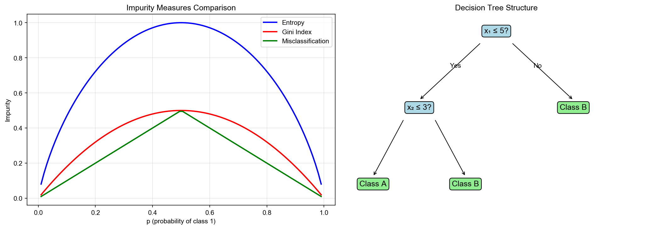
Select feature that maximizes (or equivalently, minimizes weighted Gini index).

Decision Tree Structure and Splitting Criteria

Relationship Between Entropy and Gini Index

For binary classification ( is positive class proportion), entropy and Gini index are:

Taylor expansion: Near ,

Both have similar shapes, but Gini index is computationally simpler (no logarithm). CART algorithm uses Gini index.

The following figure compares how entropy and Gini index vary with class probability:

Mean Squared Error Criterion (Regression Trees)

For regression tasks, the goal is to minimize prediction error at leaf nodes. If leaf node contains samples, prediction value is:

(i.e., mean of target values in the region)

Splitting criterion: Select feature and split point that minimize total MSE after splitting:

where , .

Optimal prediction values: Given split, optimal are region means:

Decision Tree Algorithms

ID3 Algorithm

ID3 (Iterative Dichotomiser 3) was proposed by Quinlan in 1986, using information gain as splitting criterion.

Algorithm:

Stopping conditions: If current node satisfies any of:
- All samples belong to same class
- Feature set is empty, or all samples have same values on all features (majority vote)
- Node sample count below threshold
Feature selection: Compute information gainfor each feature , select maximum:

Split: Split intobased on valuesof feature
Recurse: Recursively build subtree for each subset

C4.5 Algorithm

C4.5 improves on ID3 with:

Gain ratio: Useinstead ofto avoid favoring multi-valued features
Continuous feature handling: Discretize continuous features (see below)
Missing value handling: Allow missing feature values (see below)
Pruning: Introduce post-pruning strategy

CART Algorithm

CART (Classification and Regression Tree) is the most widely used decision tree algorithm, proposed by Breiman et al. in 1984.

Features: - Binary tree: Each split produces two child nodes (ID3/C4.5 can produce multiple) - Gini index (classification) or MSE (regression) as splitting criterion - Cost-Complexity Pruning

Classification tree splitting:

For feature and split point , split data into:

Selectthat minimizes weighted Gini index:

Regression tree splitting:

whereare target means of the two regions.

Continuous Features and Missing Values

Discretization of Continuous Features

For continuous feature , C4.5/CART uses binary split:

Sort feature values:
Consider all possible split points:
For each split point , compute criterion (Gini index or entropy)
Select optimal

Complexity: For samples, need split points, each evaluation is , total (single feature).

Optimization: Pre-sort feature values, reducing to .

Missing Value Handling

For missing values, C4.5 uses these strategies:

Strategy 1: Handling during splitting

When computing information gain, only use non-missing samples:

where is the set of samples with non-missing feature , is the non-missing proportion (as weight).

Strategy 2: Handling during sample partitioning

For samples with missing feature , distribute proportionally to all child nodes:

where is sample 's initial weight (usually 1), is weight assigned to child node .

Strategy 3: Handling during prediction

If test sample has missing feature : - Method 1: Follow all branches, weight-average predictions by - Method 2: Follow branch with most samples

Pruning Strategies

Why Pruning is Needed

Fully grown decision trees (until leaf nodes have only one sample or same-class samples) severely overfit: Training error is 0, but test error is high.

Causes of overfitting: - Tree too deep, captures noise in training data - Too few samples in leaf nodes, unreliable statistics

Solution: Pruning — simplify tree structure to improve generalization.

Pre-Pruning

Stop splitting early during construction. Common stopping conditions:

Node sample threshold:
Depth limit: Depth reaches
Information gain threshold:
Leaf sample threshold: Post-split child node samples

Advantages: Computationally efficient, avoids building too-deep trees

Disadvantages: May stop too early, causing underfitting (some seemingly ineffective splits may be useful later)

Post-Pruning

Build complete tree first, then prune bottom-up.

Basic idea: For internal node , compare performance on validation set before and after pruning: - Before pruning: has subtree - After pruning: becomes leaf node

If performance doesn't decrease (or improves) after pruning, then prune.

Cost-Complexity Pruning (CART pruning):

Introduce tree complexity penalty. Define tree 's cost-complexity:

where: - is training error (sum of leaf losses) - is number of leaf nodes - is complexity parameter (hyperparameter)

Physical meaning: controls tradeoff between fit and complexity. Larger favors simpler trees.

Pruning process:

Generate pruning sequence: From full tree , incrementally prune to get sequence ( is root node)

For each internal node , compute cost-complexity change:

where is subtree rooted at . Select node with smallest to prune.

Cross-validation to select optimal: Evaluate each tree in sequence on validation set, select with minimum validation error.

The following figure shows the effect of the complexity parameter on pruning, along with how training and validation errors change:

Complete Implementation

import numpy as np

class Node:
    def __init__(self, feature=None, threshold=None, left=None, right=None, 
                 value=None):
        self.feature = feature       # Split feature index
        self.threshold = threshold   # Split threshold
        self.left = left            # Left subtree
        self.right = right          # Right subtree
        self.value = value          # Leaf node prediction value

class DecisionTreeClassifier:
    def __init__(self, max_depth=None, min_samples_split=2, 
                 min_samples_leaf=1, criterion='gini'):
        self.max_depth = max_depth
        self.min_samples_split = min_samples_split
        self.min_samples_leaf = min_samples_leaf
        self.criterion = criterion
        self.root = None
        
    def gini(self, y):
        """Compute Gini index"""
        _, counts = np.unique(y, return_counts=True)
        probs = counts / len(y)
        return 1 - np.sum(probs ** 2)
    
    def entropy(self, y):
        """Compute entropy"""
        _, counts = np.unique(y, return_counts=True)
        probs = counts / len(y)
        return -np.sum(probs * np.log2(probs + 1e-10))
    
    def split_criterion(self, y):
        """Select evaluation function based on criterion"""
        if self.criterion == 'gini':
            return self.gini(y)
        elif self.criterion == 'entropy':
            return self.entropy(y)
    
    def best_split(self, X, y):
        """Find optimal split"""
        n_samples, n_features = X.shape
        if n_samples < self.min_samples_split:
            return None, None
        
        # Parent node impurity
        parent_impurity = self.split_criterion(y)
        best_gain = 0
        best_feature = None
        best_threshold = None
        
        for feature in range(n_features):
            thresholds = np.unique(X[:, feature])
            for threshold in thresholds:
                # Split
                left_mask = X[:, feature] <= threshold
                right_mask = ~left_mask
                
                if np.sum(left_mask) < self.min_samples_leaf or \
                   np.sum(right_mask) < self.min_samples_leaf:
                    continue
                
                # Compute information gain
                n_left, n_right = np.sum(left_mask), np.sum(right_mask)
                left_impurity = self.split_criterion(y[left_mask])
                right_impurity = self.split_criterion(y[right_mask])
                weighted_impurity = (n_left * left_impurity + n_right * right_impurity) / n_samples
                gain = parent_impurity - weighted_impurity
                
                if gain > best_gain:
                    best_gain = gain
                    best_feature = feature
                    best_threshold = threshold
        
        return best_feature, best_threshold
    
    def build_tree(self, X, y, depth=0):
        """Recursively build decision tree"""
        n_samples, n_features = X.shape
        n_classes = len(np.unique(y))
        
        # Stopping conditions
        if n_classes == 1 or \
           (self.max_depth is not None and depth >= self.max_depth):
            leaf_value = np.argmax(np.bincount(y))
            return Node(value=leaf_value)
        
        # Find optimal split
        feature, threshold = self.best_split(X, y)
        if feature is None:
            leaf_value = np.argmax(np.bincount(y))
            return Node(value=leaf_value)
        
        # Recursively build subtrees
        left_mask = X[:, feature] <= threshold
        right_mask = ~left_mask
        left_subtree = self.build_tree(X[left_mask], y[left_mask], depth + 1)
        right_subtree = self.build_tree(X[right_mask], y[right_mask], depth + 1)
        
        return Node(feature=feature, threshold=threshold, 
                    left=left_subtree, right=right_subtree)
    
    def fit(self, X, y):
        """Train model"""
        self.root = self.build_tree(X, y)
        return self
    
    def predict_sample(self, x, node):
        """Predict single sample"""
        if node.value is not None:
            return node.value
        
        if x[node.feature] <= node.threshold:
            return self.predict_sample(x, node.left)
        else:
            return self.predict_sample(x, node.right)
    
    def predict(self, X):
        """Predict multiple samples"""
        return np.array([self.predict_sample(x, self.root) for x in X])

The following figure shows how decision tree depth affects overfitting — as depth increases, the decision boundary becomes more complex, transitioning from underfitting to overfitting:

The following animation shows the CART algorithm progressively splitting the feature space, selecting the optimal split point at each step:

The following figure shows the feature importance ranking from a decision tree trained on the Iris dataset:

Q&A Highlights

Q1: Why can decision trees handle nonlinear problems?

A: Decision trees recursively partition feature space into multiple rectangular regions, each corresponding to a leaf node prediction. Although each split is linear (), combinations of multiple splits can approximate arbitrarily complex nonlinear decision boundaries. This is similar to approximating continuous functions with piecewise constant functions.

Q2: Why does information gain tend to favor multi-valued features?

A: Extreme case: If feature is sample ID (unique for each sample), splitting by ID puts one sample in each subset, , information gain reaches maximum . But such splits have no generalization ability. The reason is information gain doesn't penalize feature complexity (number of values). Gain ratio solves this by dividing by .

Q3: Which is better, Gini index or entropy?

A: Theoretically equivalent (both concave functions with similar shapes), but slight practical differences: - Gini index: Faster computation (no logarithm), used by CART - Entropy: Better fits information theory interpretation, used by ID3/C4.5

Experiments show performance differences are small. Choice mainly based on computational efficiency and implementation preference.

Q4: How to handle categorical features?

A: For unordered categories (e.g., color: red, green, blue): - Method 1: One-Hot encoding, convert to multiple binary features - Method 2: Multi-way split (ID3 style), one branch per category value - Method 3: Binary split (CART style), divide categories into two subsets (need to traversepartitions, is category count)

For ordered categories (e.g., level: low, medium, high), treat as continuous feature.

Q5: Can decision trees handle multi-output tasks?

A: Yes. For multi-output regression (e.g., predict both height and weight), leaf nodes store mean of target vectors:

For multi-label classification, leaf nodes store probability distributions for each label.

Q6: Which is better, pre-pruning or post-pruning?

A: - Pre-pruning: Fast, but may stop too early (some seemingly ineffective splits may be useful later) - Post-pruning: More accurate (based on complete tree information), but higher computational cost

In practice, pre-pruning for quick prototypes, post-pruning for fine-tuning. Scikit-learn decision trees mainly use pre-pruning.

Q7: Why are decision trees insensitive to feature scales?

A: Decision tree split condition is , only comparing relative order, not involving distance computation. Even if feature rangesand ranges, only which side samples fall on matters, not affected by scale. This differs from distance-based algorithms (like KNN, SVM).

✏️ Exercises and Solutions

Exercise 1: Information Gain Calculation

Problem: Dataset has 14 samples, 9 positive and 5 negative. Feature has two values: when there are 8 samples (6 positive, 2 negative), when there are 6 samples (3 positive, 3 negative). Compute the information gain and gain ratio of feature .

Solution:

Parent node entropy:

Child node entropies:

Conditional entropy:

Information gain:

Intrinsic value:

Gain ratio:

Exercise 2: Gini Index and Entropy Approximation

Problem: Prove that for binary classification with natural logarithm, near . (Hint: Taylor expansion at )

Solution:

Let. Taylor expansion of entropy around :

Gini index:

Their ratio near :

Thus . When using, the maximum values are and, giving .

Exercise 3: Cost-Complexity Pruning

Problem: A decision tree has subtree with 4 leaf nodes. The subtree's training error is , and the pruned node's training error is . Compute the critical and determine whether to prune when.

Solution:

Critical value:

When: - Without pruning: - With pruning:

Since, pruning yields lower cost-complexity, so we should prune. Intuitively, when exceeds the critical value, the complexity penalty is strong enough that the subtree's improved fit doesn't justify its added complexity.

Exercise 4: Missing Value Correction

Problem: Dataset has 100 samples, feature has 20 missing values. Among the 80 non-missing samples, and after splitting. Compute the corrected information gain.

Solution:

Non-missing proportion:

Corrected information gain:

More missing values lead to smaller and thus larger correction. This naturally penalizes features with high missing rates, since less information is available for reliable splitting.

Exercise 5: Multivariate Decision Trees

Problem: A standard decision tree (univariate splits) creates "staircase" decision boundaries in 2D. How many splits are needed to approximate the line ? How about a multivariate decision tree?

Solution:

Standard decision tree: Each split produces axis-aligned boundaries ( or ). To approximate the diagonal , multiple "staircase" steps are needed. To control approximation error below, roughly splits are required (e.g., needs about 10 splits).

Multivariate decision tree: Using linear combination with , only 1 split is needed to exactly represent .

This is the advantage of multivariate decision trees: more compact trees for diagonal boundaries. The trade-off is that finding optimalrequires solving an optimization problem, which is more computationally expensive.

References

Quinlan, J. R. (1986). Induction of decision trees. Machine Learning, 1(1), 81-106.
Quinlan, J. R. (1993). C4.5: Programs for Machine Learning. Morgan Kaufmann.
Breiman, L., Friedman, J., Stone, C. J., & Olshen, R. A. (1984). Classification and Regression Trees. Wadsworth.
Hastie, T., Tibshirani, R., & Friedman, J. (2009). The Elements of Statistical Learning (2nd ed.). Springer. [Chapter 9: Additive Models, Trees, and Related Methods]
Mitchell, T. M. (1997). Machine Learning. McGraw-Hill. [Chapter 3: Decision Tree Learning]
Breiman, L. (2001). Random forests. Machine Learning, 45(1), 5-32.

Decision trees, with their intuitive structure and powerful expressive capability, are important tools in machine learning. From information entropy to Gini index, from ID3 to CART, this chapter systematically derives theoretical foundations and algorithm details of decision trees. Understanding decision trees is not only needed for mastering classical algorithms, but prerequisite for understanding ensemble learning (Random Forest, GBDT, XGBoost)— these modern algorithms all center on combining and optimizing decision trees.