The leap from linear regression to logistic regression marks an important transition in machine learning from regression to classification tasks. Although named "regression," logistic regression is fundamentally a classification algorithm, establishing a bridge between linear models and probability predictions through the Sigmoid function. This chapter delves into the mathematical essence of logistic regression: from likelihood function construction to gradient computation details, from binary to multi-class extension, from optimization algorithms to regularization techniques, comprehensively revealing the probabilistic modeling approach to classification.

From Linear Models to Probabilistic Classification

Limitations of Linear Classification

Recall linear regression, which establishes a linear mapping between inputs and continuous outputs:

But classification task labels are discrete (e.g.,), and using linear models directly has two problems:

Unconstrained output:can be any real number, but class labels must be in a finite set
Missing probability interpretation: Linear models cannot give "probability that sample belongs to a class"

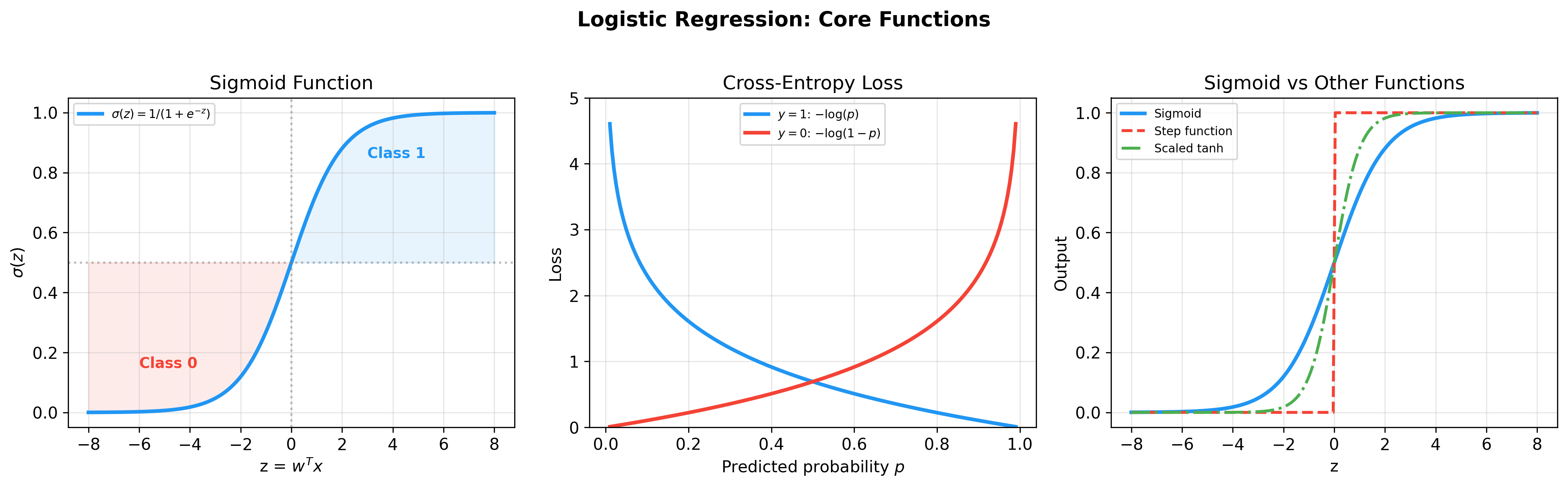
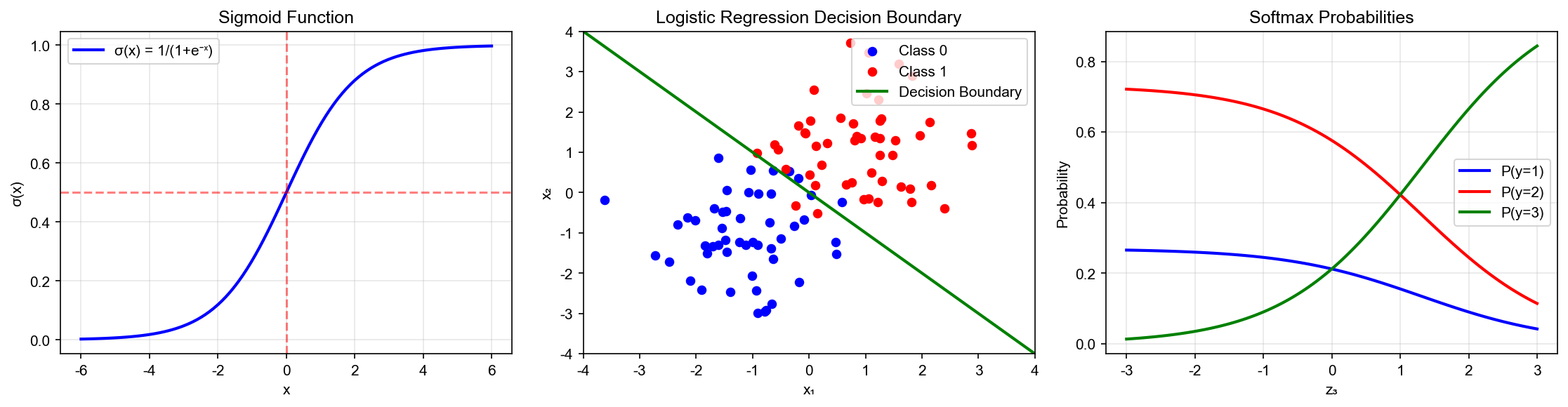
Logistic regression solves this contradiction by introducing a link function: mapping the linear model output to theinterval, giving it probabilistic meaning.

Sigmoid Function: From Real Numbers to Probabilities

The Sigmoid function is defined as:

It has elegant mathematical properties:

Property 1: Range Constraint

For any, we have, satisfying probability requirements.

Property 2: Symmetry

Proof:

Property 3: Self-Expressing Derivative

Proof:

This property is key to the simplicity of gradient computation.

Logistic Regression Model Definition

For binary classification (), define:

Correspondingly:

Unified Representation: Using exponential form, both probabilities can be combined as:

When, the formula reduces to; when, it reduces to.

Maximum Likelihood Estimation and Loss Function

Likelihood Function Construction

Given training set, assuming samples are independent and identically distributed (i.i.d.), the likelihood function is:

Substituting the logistic regression model:

Log-Likelihood and Cross-Entropy

Taking logarithm gives log-likelihood:

Maximizing log-likelihood is equivalent to minimizing negative log-likelihood:

whereis the predicted probability. This is the Binary Cross-Entropy Loss.

Information Theory Interpretation: Cross-entropy measures the difference between true distributionand predicted distribution:

In binary classification, true distributioncorresponds to hard labels, predicted distributioncorresponds to, substituting gives the loss above.

Comparison with Mean Squared Error

If using MSE as loss:

Computing gradient:

Note the extra term. Whenis close to 0 or 1 (i.e., model is very confident), this term approaches 0, causing vanishing gradients— even if prediction is wrong, almost no update occurs.

Cross-entropy loss gradient (derived below) is:

Without theterm, avoiding the vanishing gradient problem.

Gradient Derivation and Optimization Algorithms

Exact Gradient Computation

For single sample loss:

where,. Using chain rule:

Step 1:

Step 2: Using Sigmoid derivative property

Step 3:

Combining:

Total gradient:

whereis the data matrix,are predicted and true label vectors.

Hessian Matrix and Second-Order Methods

For second-order optimization like Newton's method, we need the Hessian matrix:

Taking derivative of single-sample gradientagain:

Total Hessian:

where.

Positive Definiteness Analysis: For any,

Since(Sigmoid output is in). Thereforeis positive definite, and loss functionis strictly convex, with a unique global optimum.

Gradient Descent and Stochastic Optimization

Batch Gradient Descent (BGD):

Stochastic Gradient Descent (SGD): Randomly select one sampleeach time,

Mini-batch Gradient Descent: Select batch sizeeach time,

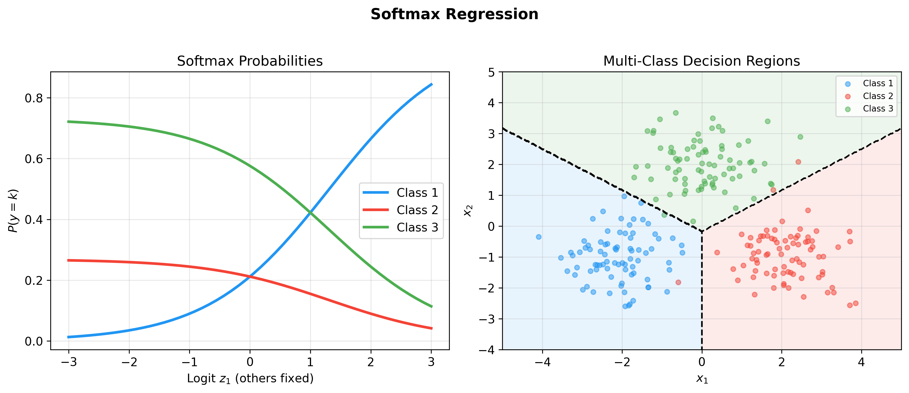
Multi-class Extension: Softmax Regression

From Binary to Multi-class

For-class classification (), we need to learn a weight vectorfor each class. Define the score for class:

Use Softmax function to normalize scores into probabilities:

whereis the parameter matrix.

Normalization Verification:

Cross-Entropy Loss and One-Hot Encoding

Introduce One-Hot encoding: If true class is, then(only positionis 1). Loss function:

where.

Simplification: Since each sample has only one(say class), rest are 0,

This is the Negative Log-Likelihood (NLL) for multi-class.

Softmax Gradient Derivation

For single-sample loss, compute gradient with respect to:

First term: $𝟙$

Second term:

Combining:

$𝟙$

Further differentiating with respect to:

Total gradient:

Matrix form:

whereare true and predicted One-Hot matrices.

Regularization Techniques

L2 Regularization (Ridge Logistic Regression)

Add L2 penalty:

Gradient becomes:

Update formula:

Theterm produces weight decay effect.

L1 Regularization (Lasso Logistic Regression)

Add L1 penalty:

L1 norm is not differentiable at 0, use subgradient:

where(when), or(when).

Sparsity: L1 regularization tends to produce sparse solutions (many weights exactly zero), achieving feature selection.

Elastic Net

Combining L1 and L2:

Combining sparsity with stability.

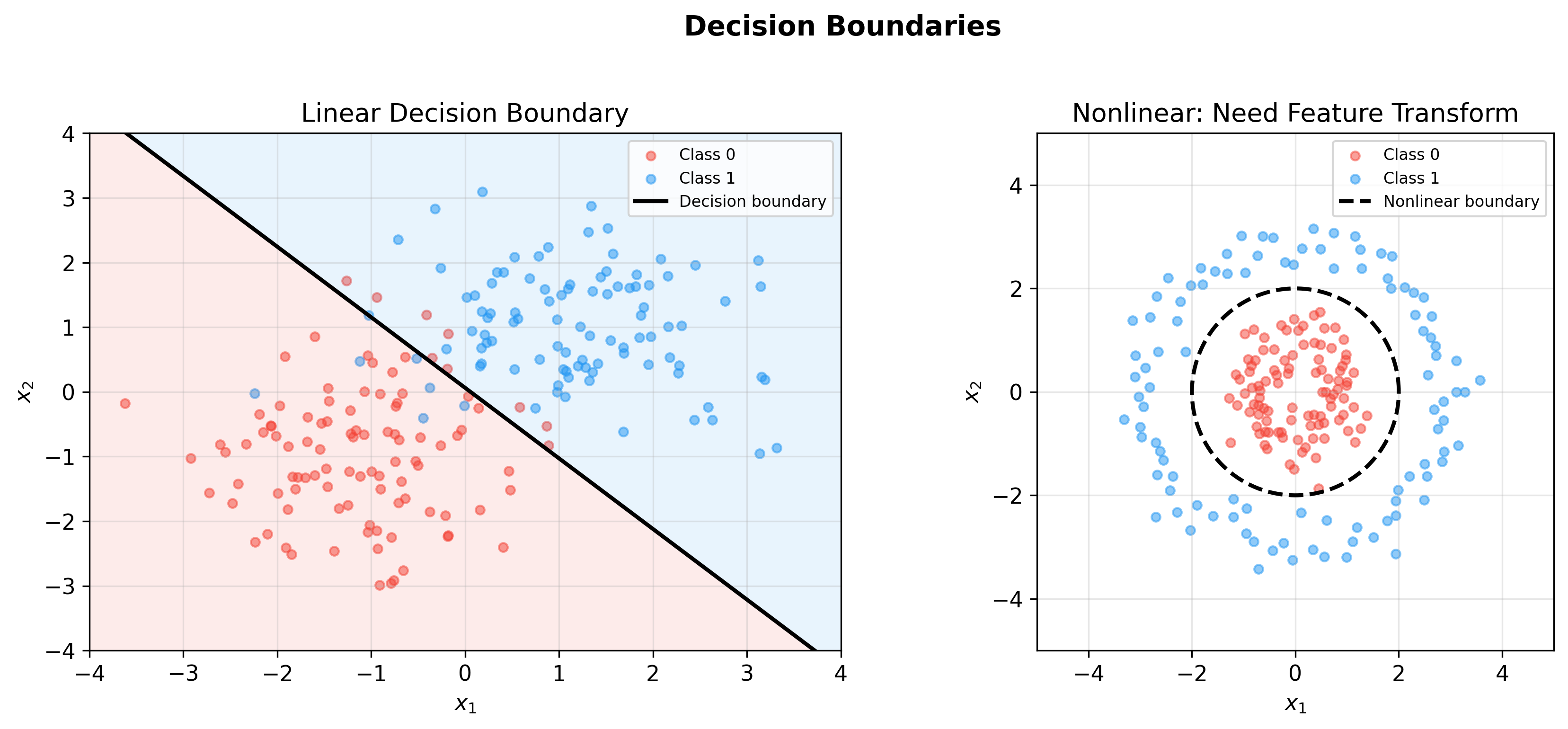
Decision Boundary and Geometric Interpretation

Binary Classification Decision Boundary

Logistic regression decision rule:

Since, the decision boundary is:

This is a hyperplane in feature space.

Distance to Boundary: For sample, its signed distance to the decision boundary is:

The larger the distance, the more confident the classification.

Multi-class Decision Regions

In-class classification, the boundary between classand classis:

Feature space is divided intoregions, each corresponding to a class. Boundaries between adjacent regions are linear.

Model Evaluation and Diagnostics

Confusion Matrix and Performance Metrics

For binary classification, define:

TP (True Positive): True positive, predicted positive
FP (False Positive): True negative, predicted positive
TN (True Negative): True negative, predicted negative
FN (False Negative): True positive, predicted negative

Accuracy:

Precision:

Recall:

F1 Score:

ROC Curve and AUC

Varying decision threshold(classifies as positive), we get different (FPR, TPR) pairs:

True Positive Rate (TPR):
False Positive Rate (FPR): ROC Curve: Curve with FPR as x-axis, TPR as y-axis.

AUC (Area Under Curve): Area under ROC curve, measures ranking ability. AUC=1 is perfect classifier, AUC=0.5 is random guessing.

Probabilistic Interpretation: AUC equals the probability that a randomly selected positive sample scores higher than a randomly selected negative sample.

Implementation Details and Numerical Stability

Sigmoid Function Numerical Overflow

Whenis very large,approaches 0, but computingmay overflow. Stable implementation:

def stable_sigmoid(z):
    if z >= 0:
        return 1 / (1 + np.exp(-z))
    else:
        exp_z = np.exp(z)
        return exp_z / (1 + exp_z)

Softmax Numerical Stability

Direct computation ofmay overflow. Using Softmax's shift invariance:

Taking:

def stable_softmax(z):
    z_max = np.max(z, axis=-1, keepdims=True)
    exp_z = np.exp(z - z_max)
    return exp_z / np.sum(exp_z, axis=-1, keepdims=True)

Complete Training Code

import numpy as np

class LogisticRegression:
    def __init__(self, learning_rate=0.01, n_iterations=1000, 
                 regularization='l2', lambda_reg=0.01):
        self.lr = learning_rate
        self.n_iter = n_iterations
        self.reg = regularization
        self.lambda_reg = lambda_reg
        self.w = None
        
    def sigmoid(self, z):
        return np.where(z >= 0, 
                        1 / (1 + np.exp(-z)),
                        np.exp(z) / (1 + np.exp(z)))
    
    def fit(self, X, y):
        N, d = X.shape
        self.w = np.zeros(d)
        
        for _ in range(self.n_iter):
            # Forward pass
            z = X @ self.w
            y_hat = self.sigmoid(z)
            
            # Compute gradient
            grad = X.T @ (y_hat - y) / N
            
            # Add regularization
            if self.reg == 'l2':
                grad += self.lambda_reg * self.w
            elif self.reg == 'l1':
                grad += self.lambda_reg * np.sign(self.w)
            
            # Gradient descent
            self.w -= self.lr * grad
    
    def predict_proba(self, X):
        return self.sigmoid(X @ self.w)
    
    def predict(self, X, threshold=0.5):
        return (self.predict_proba(X) >= threshold).astype(int)

# Example usage
if __name__ == '__main__':
    from sklearn.datasets import make_classification
    from sklearn.model_selection import train_test_split
    from sklearn.metrics import accuracy_score, roc_auc_score
    
    # Generate data
    X, y = make_classification(n_samples=1000, n_features=20, 
                                n_informative=15, n_redundant=5, 
                                random_state=42)
    X_train, X_test, y_train, y_test = train_test_split(
        X, y, test_size=0.2, random_state=42)
    
    # Train model
    model = LogisticRegression(learning_rate=0.1, n_iterations=1000, 
                                regularization='l2', lambda_reg=0.01)
    model.fit(X_train, y_train)
    
    # Evaluate
    y_pred = model.predict(X_test)
    y_prob = model.predict_proba(X_test)
    
    print(f"Accuracy: {accuracy_score(y_test, y_pred):.4f}")
    print(f"AUC: {roc_auc_score(y_test, y_prob):.4f}")

Multi-class Implementation

class SoftmaxRegression:
    def __init__(self, learning_rate=0.01, n_iterations=1000, 
                 lambda_reg=0.01):
        self.lr = learning_rate
        self.n_iter = n_iterations
        self.lambda_reg = lambda_reg
        self.W = None
        
    def softmax(self, Z):
        """Stable Softmax computation"""
        Z_max = np.max(Z, axis=1, keepdims=True)
        exp_Z = np.exp(Z - Z_max)
        return exp_Z / np.sum(exp_Z, axis=1, keepdims=True)
    
    def fit(self, X, y):
        N, d = X.shape
        K = len(np.unique(y))
        self.W = np.zeros((d, K))
        
        # Convert to One-Hot encoding
        Y_one_hot = np.zeros((N, K))
        Y_one_hot[np.arange(N), y] = 1
        
        for _ in range(self.n_iter):
            # Forward pass
            Z = X @ self.W
            Y_hat = self.softmax(Z)
            
            # Compute gradient
            grad = X.T @ (Y_hat - Y_one_hot) / N
            grad += self.lambda_reg * self.W  # L2 regularization
            
            # Update weights
            self.W -= self.lr * grad
    
    def predict_proba(self, X):
        Z = X @ self.W
        return self.softmax(Z)
    
    def predict(self, X):
        return np.argmax(self.predict_proba(X), axis=1)

# Example usage
if __name__ == '__main__':
    from sklearn.datasets import make_classification
    from sklearn.model_selection import train_test_split
    from sklearn.metrics import accuracy_score
    
    # Generate multi-class data
    X, y = make_classification(n_samples=1000, n_features=20, 
                                n_informative=15, n_redundant=5,
                                n_classes=5, random_state=42)
    X_train, X_test, y_train, y_test = train_test_split(
        X, y, test_size=0.2, random_state=42)
    
    # Train model
    model = SoftmaxRegression(learning_rate=0.1, n_iterations=1000, 
                               lambda_reg=0.01)
    model.fit(X_train, y_train)
    
    # Evaluate
    y_pred = model.predict(X_test)
    print(f"Accuracy: {accuracy_score(y_test, y_pred):.4f}")

Q&A Highlights

Q1: Why called "logistic regression" instead of "logistic classification"?

A: Historical reasons. Logistic regression was originally used for probabilistic modeling in regression problems, mapping linear model output to probability through the Logistic function (i.e., Sigmoid). Later it was found more suitable for classification, but the name persists.

Q2: What is the essential difference between logistic and linear regression?

A: The core difference lies in output space and loss function: - Linear regression:, uses MSE loss, assumes noise follows Gaussian distribution - Logistic regression:, uses cross-entropy loss, assumes labels follow Bernoulli distribution

Both are special cases of Generalized Linear Models (GLM), differing only in link function and assumed distribution.

Q3: Why is cross-entropy better than MSE for classification?

A: MSE gradient contains theterm; when prediction is very confident (or) but wrong, gradient approaches 0, barely updating. Cross-entropy gradient is; even confident but wrong predictions produce large gradients for quick correction.

Q4: Can logistic regression fit nonlinear boundaries?

A: Original logistic regression is a linear classifier with hyperplane decision boundary. But through: - Feature engineering: Adding polynomial features (e.g.,) - Kernel methods: Implicitly mapping to high-dimensional space - Neural networks: Stacking multiple logistic regression layers

nonlinear classification can be achieved.

Q5: Difference between Softmax and multiple independent Sigmoids?

A: - Softmax: Class probabilities are normalized,, for mutually exclusive multi-class (single label) - Multiple Sigmoids: Each label is independent, probability sum can be, for multi-label classification

For example, news classification (single category) uses Softmax; tag recommendation (multi-label) uses multiple Sigmoids.

Q6: How to choose regularization parameter?

A: Through cross-validation grid search: 1. Candidate values: 2. For each, evaluate performance on validation set 3. Selectwith minimum validation error

Generally, largermeans simpler model (underfitting risk), smallermeans more complex (overfitting risk).

Q7: Why is logistic regression a convex optimization problem?

A: Hessian matrixis positive definite (diagonal elements ofsatisfy), so loss function is strictly convex. Convexity guarantees: - Any local optimum is global optimum - Gradient descent and similar algorithms must converge

This is an important advantage of logistic regression.

Q8: Can logistic regression handle missing values?

A: Standard logistic regression doesn't directly support this. Common approaches: - Deletion: Delete samples with missing values (loses information) - Imputation: Fill with mean/median/mode - Indicator variables: Add binary indicator for missing features - Model prediction: Predict missing values using other features

Or use algorithms that support missing values (like XGBoost).

Q9: Why is feature standardization needed?

A: Different feature scales (e.g., age [0,100] vs income [0,1e6]) cause: 1. Large numerical range differences in gradients, requiring very small learning rate 2. Some features dominate weight updates 3. Unfair regularization (penalizes large-scale features)

Standardization () makes all features same scale, optimization more stable.

Q10: Difference between logistic regression and SVM?

A: | Dimension | Logistic Regression | SVM | |-----------|--------------------|----| | Loss | Cross-Entropy | Hinge Loss | | Output | Probability | Decision value | | Support vectors | All samples participate | Only boundary samples | | Kernel trick | Not directly supported | Naturally supported | | Convexity | Strictly convex | Convex |

Logistic regression suits probability prediction; SVM suits hard classification and nonlinear boundaries.

Q11: How to interpret logistic regression coefficients?

A: Weight represents the effect of feature on log-odds:

-: Asincreases, positive class probability increases -: Asincreases, negative class probability increases - Larger: Stronger effect

Odds ratio: Whenincreases by 1 unit, odds multiply by.

Q12: What is the time complexity of logistic regression?

A: - Single iteration:(matrix multiplication) - Total training:,is number of iterations - Prediction:(samples)

For large-scale data, use SGD or mini-batch gradient descent, reducing single iteration to(is batch size).

✏️ Exercises and Solutions

Exercise 1: Sigmoid Function Properties

Problem: Prove thatand.

Solution:

Derivative:

Symmetry:

Exercise 2: Cross-Entropy Loss Derivation

Problem: Derive the binary cross-entropy loss from maximum likelihood estimation.

Solution:

Likelihood: where .

Negative log-likelihood gives cross-entropy:

Exercise 3: Softmax Gradient

Problem: Derivefor softmax cross-entropy loss.

Solution:

With and :

This elegant result () is identical in form to logistic regression's gradient.

Exercise 4: Regularization as Bayesian Prior

Problem: What prior distributions do L2 and L1 regularization correspond to?

Solution:

L2: Gaussian prior , since.

L1: Laplace prior , since. The sharp peak at zero explains L1's sparsity-inducing property.

Exercise 5: Decision Boundary Geometry

Problem: Prove that the decision boundary is a hyperplane, and explain how and determine it.

Solution:

This is a hyperplane with normal vector and offset : - direction determines the hyperplane orientation - determines transition sharpness — largermeans steeper transition from to - Distance from point to boundary: , and

References

Bishop, C. M. (2006). Pattern Recognition and Machine Learning. Springer. [Chapter 4: Linear Models for Classification]
Hastie, T., Tibshirani, R., & Friedman, J. (2009). The Elements of Statistical Learning (2nd ed.). Springer. [Chapter 4: Linear Methods for Classification]
Murphy, K. P. (2012). Machine Learning: A Probabilistic Perspective. MIT Press. [Chapter 8: Logistic Regression]
Goodfellow, I., Bengio, Y., & Courville, A. (2016). Deep Learning. MIT Press. [Chapter 5: Machine Learning Basics]
Ng, A. Y., & Jordan, M. I. (2002). On discriminative vs. generative classifiers: A comparison of logistic regression and naive Bayes. Advances in Neural Information Processing Systems, 14.
Hosmer, D. W., Lemeshow, S., & Sturdivant, R. X. (2013). Applied Logistic Regression (3rd ed.). Wiley.

Logistic regression, with its concise mathematical form, clear probabilistic interpretation, and efficient optimization algorithms, becomes the baseline model for classification tasks. From Sigmoid to Softmax, from gradient descent to regularization, this chapter provides complete derivation of the theoretical framework. Understanding logistic regression is not only fundamental to mastering classical machine learning, but also the gateway to neural networks and deep learning — after all, every layer of a deep neural network contains the essence of logistic regression.