In 1886, Francis Galton discovered a peculiar phenomenon while studying the relationship between parents' and children's heights: parents with extreme heights tended to have children whose heights were closer to the average. He coined the term "regression toward the mean," which is where "regression" comes from. However, the true power of linear regression lies not in statistical description, but in its role as the mathematical foundation for almost all machine learning algorithms — from neural networks to support vector machines, all can be viewed as generalizations of linear regression.

The essence of linear regression is finding the optimal hyperplane in data space. This seemingly simple problem conceals deep connections between linear algebra, probability theory, and optimization. This chapter provides complete mathematical derivations of linear regression from multiple perspectives.

Basic Form of Linear Regression

Problem Definition

Given training dataset, where:

-is a-dimensional input vector (features) -is the scalar output (target value)

Objective: Find parameter vectorand biassuch that the linear model:

best fits the training data.

Notation Simplification: To unify notation, we absorb the bias into the weight vector. Define the augmented feature vector:

Then the model simplifies to:

For brevity, we omit the tildes and write, understanding thatincludes the constant term 1.

Matrix Form

Organize all training samples into matrix form:

Design Matrix:

Output Vector:

Prediction Vector:

Our goal is to find optimalsuch that prediction vectoris as close as possible to true values.

Least Squares: Algebraic Derivation

Loss Function

Using squared loss (L2 loss) to measure prediction error:

The coefficienteliminates constants when taking derivatives.

Objective:

Gradient Derivation

Calculate the gradient of the loss function with respect to. Using the chain rule:

Expanding:

Taking derivatives with respect to (using matrix differentiation formulas):

Therefore:

Normal Equation

Setting the gradient to zero:

This is the famous Normal Equation.

Theorem 1 (Least Squares Solution): Ifis invertible, the unique solution to the least squares problem is:

Proof:

First-order necessary condition:gives
Second-order sufficient condition: Computing the Hessian matrix:

For any non-zero vector:

Ifhas full column rank (i.e.,), thenif and only if, thusis positive definite.

Positive definite Hessian + zero gradient = global minimum. QED.

Invertibility Conditions for:

Necessary and sufficient condition:has full column rank, i.e.,
Equivalent condition:is positive definite
Practical interpretation:
- Number of samples(at least as many samples as features)
- Features are linearly independent (no perfect collinearity)

Moore-Penrose Pseudoinverse

Whenis not invertible (e.g.,or collinear features), use the Pseudoinverse:

whereis the Moore-Penrose pseudoinverse.

Properties:

Whenis invertible,(degenerates to ordinary inverse) -is the minimum norm solution among all solutions satisfying:

Computation: Via Singular Value Decomposition (SVD). Let, then:

whereis the pseudoinverse of(non-zero singular values are inverted, zeros remain zero).

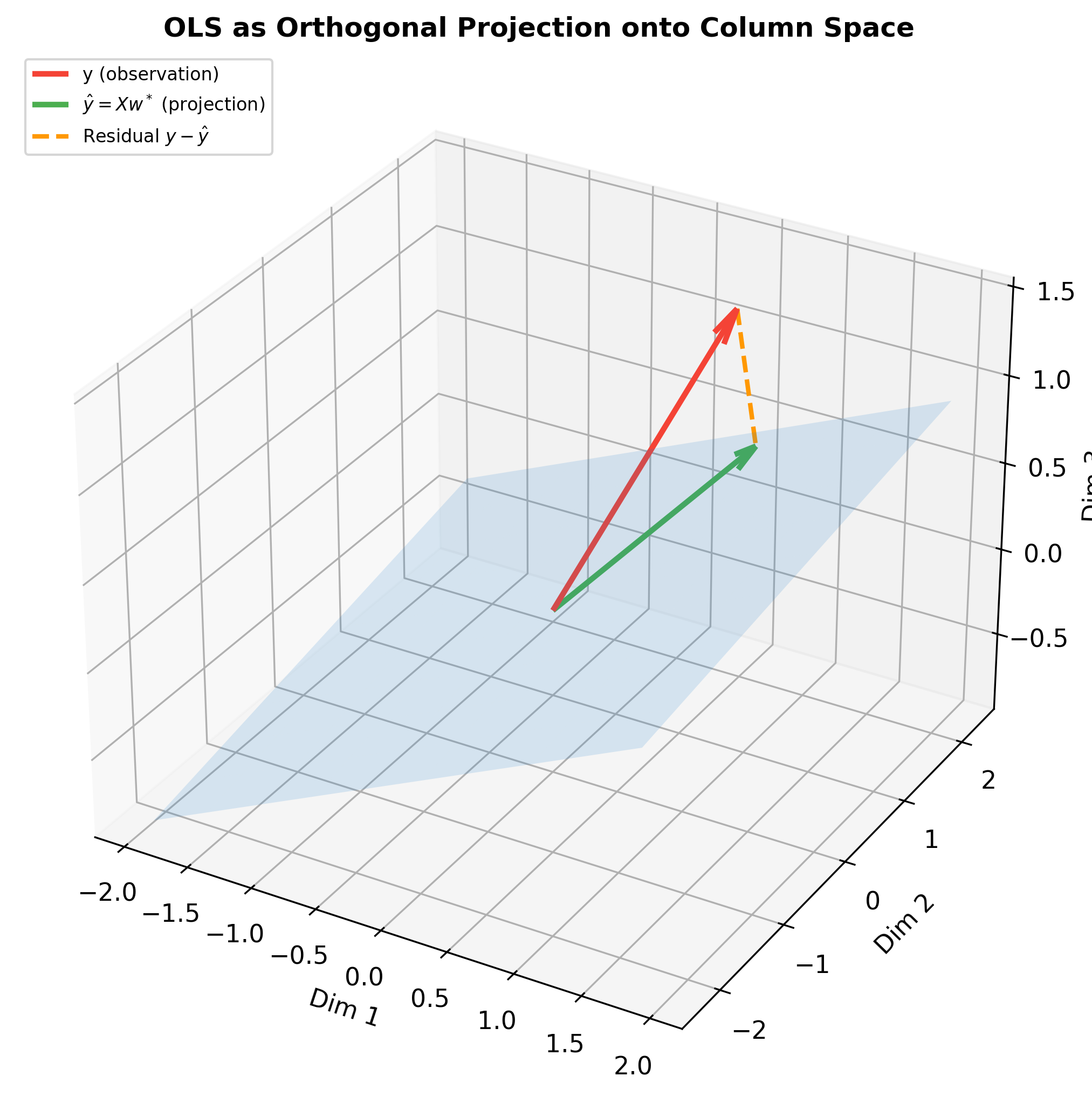
Geometric Interpretation: Projection Perspective

Column Space and Projection

The geometric essence of linear regression is orthogonal projection.

Definitions:

-is the column space of, i.e., the subspace spanned by columns of -is a vector in - The goal is to find the point inclosest to Theorem 2 (Orthogonal Projection Theorem):is the orthogonal projection ofontoif and only if the residual vectoris orthogonal to:

This is exactly the normal equation!

Proof:

For any, consider the squared norm of prediction error:

Using the Pythagorean theorem (when two vectors are orthogonal):

Let,. If, then:

Therefore:

Equality holds if and only if. QED.

Projection Matrix

Definition: The projection matrixprojects any vector onto:

Properties:

Idempotent:(projecting twice equals projecting once)
Symmetric:
Effect:is the projection ofonto the column space

Residual Projection Matrix:

Satisfying:

Properties:

-(idempotent) -(symmetric) -(residual is orthogonal to column space)

Geometric Intuition

In-dimensional space:

-is the true output vector -is a-dimensional subspace (ifhas full column rank) -is the "shadow" ofon -is the residual perpendicular to Analogy (2D plane projection):

Imagine in 3D space, the perpendicular distance from a pointto a 2D plane. The projection pointminimizes this distance.

The figure below shows OLS as orthogonal projection in 3D — observation vector is projected onto the column space of design matrix , with residual perpendicular to the column space:

Probabilistic Perspective: Maximum Likelihood Estimation

Linear Gaussian Model

Assume the data generating process is:

whereare independent and identically distributed Gaussian noise.

Equivalent form:

That is, given,follows a Gaussian distribution with meanand variance.

Likelihood Function

Given training data, the likelihood function for parametersis:

Log-Likelihood

Taking logarithm (monotonic transformation doesn't change the maximum point):

Maximum Likelihood Estimation

Optimization with respect to:

Maximizingis equivalent to minimizing:

This is exactly the least squares objective!

Theorem 3: Under the linear Gaussian model, maximum likelihood estimation is equivalent to least squares estimation:

Optimization with respect to:

Fixing, taking partial derivative with respect to:

Solving:

The MLE of noise variance is the mean of squared residuals.

Bayesian Perspective

Introducing a prior distributionon parameters, compute the posterior via Bayes' rule:

Gaussian Prior: Assuming, then:

Maximizing the posterior probability (MAP) is equivalent to minimizing:

This is the Ridge Regression objective function! The regularization termreflects the strength of prior belief.

Regularization: Ridge Regression and Lasso

Ridge Regression (L2 Regularization)

Objective Function:

whereis the regularization parameter.

Gradient:

Setting gradient to zero:

Analytical Solution:

Key Observations:

Addingguarantees invertibility of(even ifis not invertible)
When, degenerates to ordinary least squares
When,(extreme regularization)

Matrix Perspective: Ridge regression "stabilizes" the matrixby adding diagonal terms, avoiding ill-conditioning problems.

Lasso Regression (L1 Regularization)

Objective Function:

whereis the L1 norm.

Characteristics:

No analytical solution (L1 norm is not differentiable)
Requires iterative algorithms (e.g., coordinate descent, proximal gradient)
Sparsity: Some parameters are compressed exactly to zero, achieving feature selection

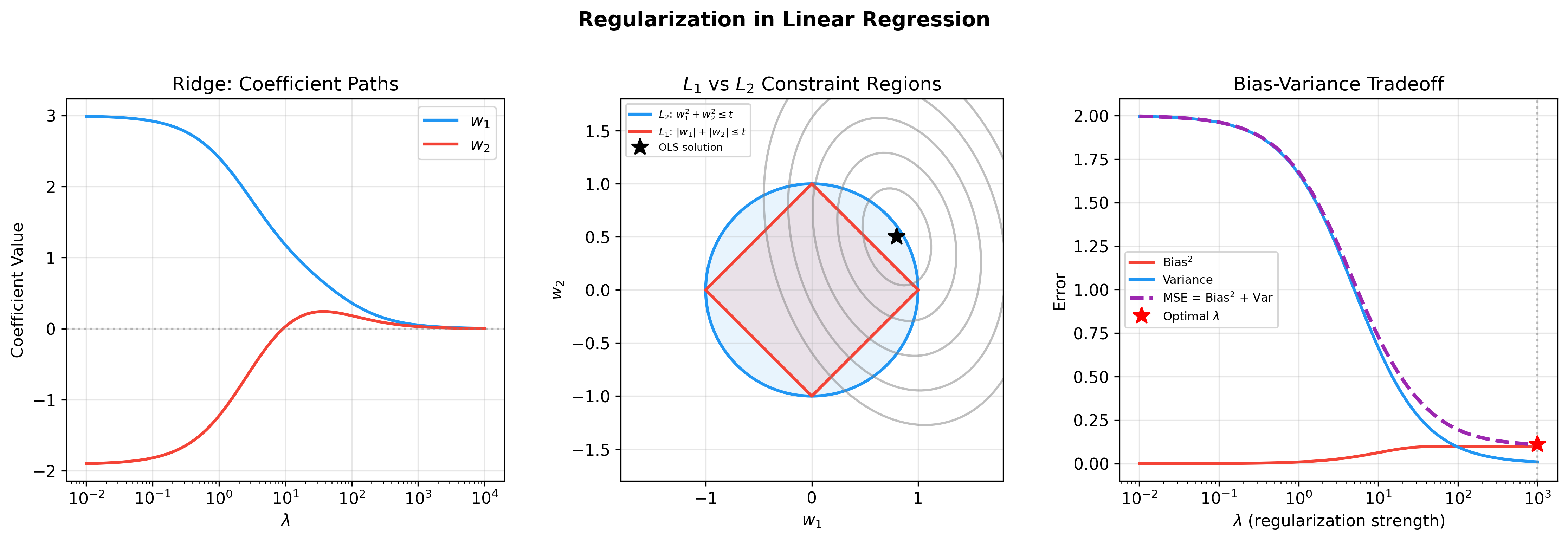
Geometric Interpretation:

In constrained form:

The L1 constraint ball is a diamond (hyperdiamond in high dimensions), whose corners are more likely to intersect with contour lines on coordinate axes, leading to sparse solutions.

Elastic Net

Combining L1 and L2:

Advantages:

Retains L1 sparsity
Retains L2 stability (friendly to collinear features)

Effects of Regularization

Bias-Variance Tradeoff:

No regularization (): Low bias, high variance (overfitting)
Strong regularization (large): High bias, low variance (underfitting)
Optimal: Selected via cross-validation

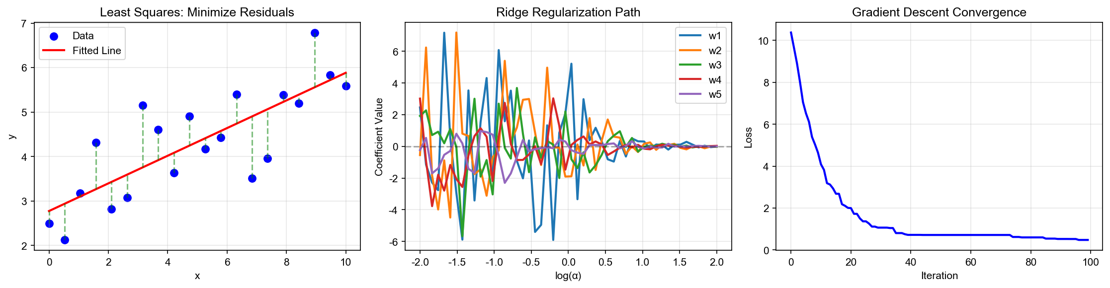
Ridge Trace:

Plotvarying withto observe shrinkage behavior of parameters.

Gradient Descent Algorithms

Batch Gradient Descent (BGD)

When data is large, directly computingis too expensive (). Use iterative algorithms.

Algorithm:

Initialize
Repeat until convergence:

whereis the learning rate, and gradient is:

Complete Form:

Computational Complexity:per iteration (matrix-vector multiplication).

Stochastic Gradient Descent (SGD)

Update parameters using only one sample at a time.

Algorithm:

Initialize
For:
- Randomly select sample - Update:

Advantages:

Fast per iteration ()
Suitable for large-scale data
Ability to escape local minima (for non-convex problems)

Disadvantages:

Unstable convergence (high variance)
Requires careful learning rate tuning

Mini-batch Gradient Descent

Compromise: Usesamples (batch size) each time.

whereis the batch at iteration(size).

Typical choices:.

Convergence Analysis

Theorem 4 (BGD Convergence): For learning rate, batch gradient descent converges linearly to the optimal solution:

where,are the minimum and maximum eigenvalues of.

Proof Sketch:

Loss function is strongly convex (Hessian is positive definite)
Gradient is Lipschitz continuous
Apply convergence theorem for strongly convex functions

Practical Recommendations:

Learning rate:(conservative choice)
Adaptive learning rates: Adam, RMSprop, etc.
Learning rate decay:

Model Evaluation and Selection

Evaluation Metrics

Mean Squared Error (MSE):

Root Mean Squared Error (RMSE):

Mean Absolute Error (MAE):

Coefficient of Determination (R ²):

whereis the mean.

Interpretation:

-: Perfect fit -: Model equivalent to predicting the mean -: Model worse than predicting the mean (rare, indicates model problems)

Adjusted R ²

Penalizing model complexity:

Advantage: Adding useless features decreases (while always increases).

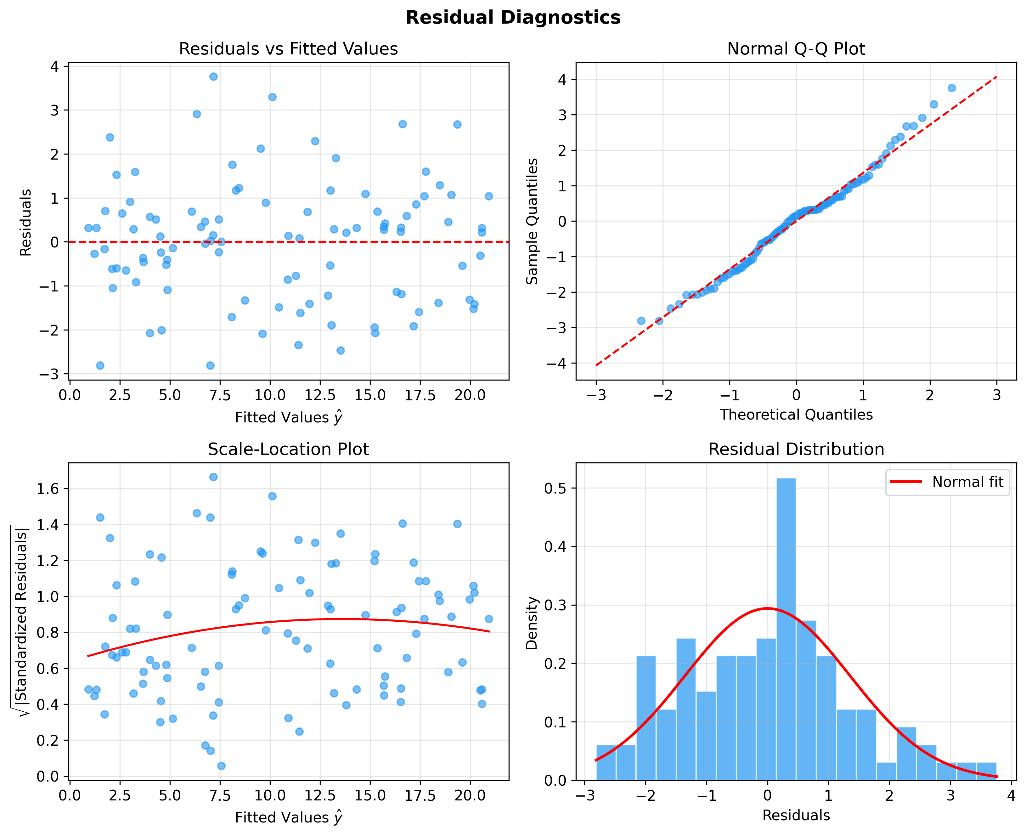
The figure below shows four classic residual diagnostic plots — residuals vs fitted values, Q-Q plot, Scale-Location plot, and residual histogram — for checking model assumptions:

Cross-Validation

k-fold Cross-Validation:

Split data intofolds
For:
- Train on all data except fold
- Test on fold
Average thetest errors

Python Implementation:

from sklearn.model_selection import cross_val_score
from sklearn.linear_model import LinearRegression

scores = cross_val_score(LinearRegression(), X, y, cv=5, 
                         scoring='neg_mean_squared_error')
rmse_scores = np.sqrt(-scores)
print(f"RMSE: {rmse_scores.mean():.4f} ± {rmse_scores.std():.4f}")

Complete Code Implementation

import numpy as np
import matplotlib.pyplot as plt
from sklearn.model_selection import train_test_split
from sklearn.preprocessing import StandardScaler

class LinearRegression:
    """
    Complete implementation of linear regression
    
    Supports:
    - Analytical solution (normal equation)
    - Batch gradient descent
    - Stochastic gradient descent
    - Ridge regularization
    """
    
    def __init__(self, method='normal', alpha=0.01, n_iterations=1000, 
                 lambda_reg=0.0, batch_size=None, random_state=42):
        """
        Parameters:
            method: str, solving method
                'normal': Normal equation
                'bgd': Batch gradient descent
                'sgd': Stochastic gradient descent
                'mini_batch': Mini-batch gradient descent
            alpha: float, learning rate (only for gradient descent)
            n_iterations: int, number of iterations
            lambda_reg: float, Ridge regularization parameter
            batch_size: int, batch size (only for mini_batch)
            random_state: int, random seed
        """
        self.method = method
        self.alpha = alpha
        self.n_iterations = n_iterations
        self.lambda_reg = lambda_reg
        self.batch_size = batch_size
        self.random_state = random_state
        self.w = None
        self.loss_history = []
        
    def fit(self, X, y):
        """
        Train linear regression model
        
        Parameters:
            X: np.array, shape=(m, d), input features
            y: np.array, shape=(m,), output labels
        """
        # Add bias term
        X_bias = self._add_bias(X)
        m, d = X_bias.shape
        
        # Initialize weights
        np.random.seed(self.random_state)
        self.w = np.random.randn(d) * 0.01
        
        if self.method == 'normal':
            # Normal equation
            self.w = self._normal_equation(X_bias, y)
        elif self.method == 'bgd':
            # Batch gradient descent
            self._batch_gradient_descent(X_bias, y)
        elif self.method == 'sgd':
            # Stochastic gradient descent
            self._stochastic_gradient_descent(X_bias, y)
        elif self.method == 'mini_batch':
            # Mini-batch gradient descent
            if self.batch_size is None:
                self.batch_size = min(32, m)
            self._mini_batch_gradient_descent(X_bias, y)
        else:
            raise ValueError(f"Unknown method: {self.method}")
        
        return self
    
    def predict(self, X):
        """
        Prediction
        
        Parameters:
            X: np.array, shape=(m, d)
        
        Returns:
            y_pred: np.array, shape=(m,)
        """
        X_bias = self._add_bias(X)
        return X_bias @ self.w
    
    def score(self, X, y):
        """
        Calculate R ² score
        """
        y_pred = self.predict(X)
        ss_res = np.sum((y - y_pred) ** 2)
        ss_tot = np.sum((y - np.mean(y)) ** 2)
        return 1 - ss_res / ss_tot
    
    def _add_bias(self, X):
        """Add bias column"""
        return np.c_[X, np.ones(X.shape[0])]
    
    def _compute_loss(self, X, y):
        """Compute loss (including regularization)"""
        m = len(y)
        predictions = X @ self.w
        mse = np.mean((predictions - y) ** 2)
        reg = self.lambda_reg * np.sum(self.w[:-1] ** 2)  # Don't regularize bias
        return mse + reg
    
    def _compute_gradient(self, X, y):
        """Compute gradient"""
        m = len(y)
        predictions = X @ self.w
        gradient = X.T @ (predictions - y) / m
        # Add regularization gradient (excluding bias)
        if self.lambda_reg > 0:
            reg_gradient = np.zeros_like(self.w)
            reg_gradient[:-1] = 2 * self.lambda_reg * self.w[:-1]
            gradient += reg_gradient
        return gradient
    
    def _normal_equation(self, X, y):
        """Solve via normal equation"""
        # w = (X^T X + lambda*I)^{-1} X^T y
        d = X.shape[1]
        reg_matrix = self.lambda_reg * np.eye(d)
        reg_matrix[-1, -1] = 0  # Don't regularize bias
        
        try:
            w = np.linalg.solve(X.T @ X + reg_matrix, X.T @ y)
        except np.linalg.LinAlgError:
            # If matrix is singular, use pseudoinverse
            w = np.linalg.pinv(X.T @ X + reg_matrix) @ X.T @ y
        
        return w
    
    def _batch_gradient_descent(self, X, y):
        """Batch gradient descent"""
        for i in range(self.n_iterations):
            gradient = self._compute_gradient(X, y)
            self.w -= self.alpha * gradient
            
            # Record loss
            if i % 10 == 0:
                loss = self._compute_loss(X, y)
                self.loss_history.append(loss)
    
    def _stochastic_gradient_descent(self, X, y):
        """Stochastic gradient descent"""
        m = len(y)
        np.random.seed(self.random_state)
        
        for i in range(self.n_iterations):
            # Randomly select one sample
            idx = np.random.randint(m)
            X_i = X[idx:idx+1]
            y_i = y[idx:idx+1]
            
            gradient = self._compute_gradient(X_i, y_i)
            self.w -= self.alpha * gradient
            
            # Record loss (every 10 iterations)
            if i % 10 == 0:
                loss = self._compute_loss(X, y)
                self.loss_history.append(loss)
    
    def _mini_batch_gradient_descent(self, X, y):
        """Mini-batch gradient descent"""
        m = len(y)
        np.random.seed(self.random_state)
        
        for i in range(self.n_iterations):
            # Randomly select batch
            indices = np.random.choice(m, self.batch_size, replace=False)
            X_batch = X[indices]
            y_batch = y[indices]
            
            gradient = self._compute_gradient(X_batch, y_batch)
            self.w -= self.alpha * gradient
            
            # Record loss
            if i % 10 == 0:
                loss = self._compute_loss(X, y)
                self.loss_history.append(loss)


# Example: Housing Price Prediction
def demo_linear_regression():
    """
    Complete example: Linear regression application on simulated housing data
    """
    # Generate synthetic data (simulating house price prediction)
    np.random.seed(42)
    m = 500
    d = 5
    
    # True weights
    w_true = np.array([50, -20, 30, 15, -10, 200])  # Last one is bias
    
    # Generate features (standardized)
    X = np.random.randn(m, d)
    
    # Add bias and compute true values
    X_bias = np.c_[X, np.ones(m)]
    y_true = X_bias @ w_true
    
    # Add noise
    noise = np.random.randn(m) * 20
    y = y_true + noise
    
    # Split training and test sets
    X_train, X_test, y_train, y_test = train_test_split(
        X, y, test_size=0.2, random_state=42
    )
    
    # Standardize
    scaler = StandardScaler()
    X_train_scaled = scaler.fit_transform(X_train)
    X_test_scaled = scaler.transform(X_test)
    
    # Compare different methods
    methods = {
        'Normal Equation': LinearRegression(method='normal'),
        'Batch GD': LinearRegression(method='bgd', alpha=0.1, n_iterations=1000),
        'SGD': LinearRegression(method='sgd', alpha=0.01, n_iterations=2000),
        'Mini-batch GD': LinearRegression(method='mini_batch', alpha=0.05, 
                                         n_iterations=1000, batch_size=32)
    }
    
    results = {}
    
    print("=" * 70)
    print("Linear Regression Method Comparison")
    print("=" * 70)
    
    for name, model in methods.items():
        # Train
        model.fit(X_train_scaled, y_train)
        
        # Evaluate
        train_score = model.score(X_train_scaled, y_train)
        test_score = model.score(X_test_scaled, y_test)
        y_pred = model.predict(X_test_scaled)
        rmse = np.sqrt(np.mean((y_test - y_pred) ** 2))
        
        results[name] = {
            'train_r2': train_score,
            'test_r2': test_score,
            'rmse': rmse,
            'weights': model.w
        }
        
        print(f"\n{name}:")
        print(f"  Training R ²: {train_score:.4f}")
        print(f"  Test R ²: {test_score:.4f}")
        print(f"  Test RMSE: {rmse:.2f}")
    
    # Ridge Regression: Effect of regularization
    print("\n" + "=" * 70)
    print("Ridge Regression: Regularization Parameter Selection")
    print("=" * 70)
    
    lambdas = [0, 0.01, 0.1, 1, 10, 100]
    train_scores = []
    test_scores = []
    
    for lam in lambdas:
        model = LinearRegression(method='normal', lambda_reg=lam)
        model.fit(X_train_scaled, y_train)
        train_scores.append(model.score(X_train_scaled, y_train))
        test_scores.append(model.score(X_test_scaled, y_test))
        print(f"λ={lam:6.2f}: Training R ²={train_scores[-1]:.4f}, "
              f"Test R ²={test_scores[-1]:.4f}")


if __name__ == "__main__":
    demo_linear_regression()

Q&A: Core Linear Regression Questions

Q1: Why use squared loss instead of absolute value loss?

Mathematical Reasons:

Differentiability:is differentiable everywhere, facilitating optimization
Analytical solution: Squared loss leads to quadratic optimization problem with closed-form solution
Statistical significance: Under Gaussian noise assumption, squared loss corresponds to maximum likelihood estimation

Absolute Value Loss (L1 loss): - Advantages: Robust to outliers (less affected by outliers) - Disadvantages: Not differentiable at zero, no analytical solution, requires linear programming

Comparison:

Loss Function	Differentiability	Analytical Solution	Outlier Robustness	Noise Distribution
Squared (L2)	Everywhere	Yes	Weak	Gaussian
Absolute (L1)	Not at 0	No	Strong	Laplacian
Huber	Everywhere	No	Medium	Mixed

Huber Loss (compromise):

Quadratic when, linear when, combining advantages of both.

Q2: Normal equation vs gradient descent — when to use which?

Decision Tree:

Data Scale?
├─ Small scale (m < 10000, d < 1000)
│  └─ Use normal equation (fast, high precision)
└─ Large scale (m > 10000 or d > 1000)
   ├─ X^T X invertible?
   │  ├─ Yes → Gradient descent
   │  └─ No → Ridge regression or gradient descent
   └─ Enough memory?
      ├─ Yes → Batch gradient descent
      └─ No → SGD or Mini-batch GD

Detailed Comparison:

Dimension	Normal Equation	Gradient Descent
Time Complexity		(is iterations)
Space Complexity
Convergence	One step	Requires multiple iterations
Hyperparameters	None	Learning rate, iterations
Feature Count	feasible	Arbitrary
Invertibility	must be invertible	Not required
Regularization	Easy to add	Easy to add
Online Learning	Not supported	Supported (SGD)

Practical Recommendations:

Default choice: Use normal equation for, otherwise gradient descent
Big data: Must use SGD or Mini-batch GD
Real-time updates: Must use SGD (supports online learning)

Q3: Why does Ridge regression solution always exist?

Core Reason: Addingmakes the matrix positive definite.

Theorem: For any, the matrixis positive definite, hence invertible.

Proof:

For any non-zero vector:

Since, we have. Even if(is in the null space of), due to:

Thereforeis positive definite, hence invertible.

Intuition:

-may be singular (e.g., collinear features) - Addingis like adding a "safety cushion" to the diagonal - Even if some features are perfectly correlated,ensures positive definiteness

Geometric Interpretation:

In feature space, the null space ofcorresponds to directions that cannot be determined from data. Ridge regression, by adding, imposes a "prefer zero" prior in these directions, making the problem well-posed.

Q4: How to choose regularization parameter?

Method 1: Cross-Validation (Recommended)

from sklearn.linear_model import RidgeCV

# Automatically select optimal lambda
lambdas = np.logspace(-3, 3, 50)
model = RidgeCV(alphas=lambdas, cv=5)
model.fit(X_train, y_train)
print(f"Optimal λ: {model.alpha_:.4f}")

Method 2: Grid Search

from sklearn.model_selection import GridSearchCV
from sklearn.linear_model import Ridge

param_grid = {'alpha': np.logspace(-3, 3, 20)}
grid = GridSearchCV(Ridge(), param_grid, cv=5, scoring='neg_mean_squared_error')
grid.fit(X_train, y_train)
print(f"Optimal λ: {grid.best_params_['alpha']:.4f}")

Method 3: Theoretical Guidance

Based on bias-variance tradeoff:

whereis noise variance,is true parameters.

Practical Experience:

Starting point:(on standardized data)
Range:(logarithmic scale search)
Fine-tuning: Narrow range around optimal value
Early stopping: Stop if validation error keeps increasing

L-curve Method:

Plotvs, selectat the "elbow" of the curve.

Q5: Why is feature standardization important?

Problem: Different feature scales cause:

Slow GD convergence: Parameter space is ellipsoidal, gradient doesn't point to optimum
Unfair regularization:penalizes large-scale features more

Example:

Suppose two features:

-: Area (range 0-1000 sqm) -: Room count (range 1-10)

Weights,may have same impact, butmainly penalizes.

Standardization Methods:

Z-score Standardization (Recommended):

where,.

Min-Max Standardization:

Effect Comparison:

Method	Mean	Std/Range	Outlier Sensitivity
Raw data	Any	Any	-
Z-score	0	1	Medium
Min-Max	-	[0,1]	High

Code:

from sklearn.preprocessing import StandardScaler

scaler = StandardScaler()
X_train_scaled = scaler.fit_transform(X_train)
X_test_scaled = scaler.transform(X_test)  # Use training set mean and std

Note: After standardization, weight interpretation changes. To recover original-scale weights:

Q6: How does multicollinearity affect linear regression?

Definition: Multicollinearity refers to high linear correlation among features.

Detection Method:

Variance Inflation Factor (VIF):

whereis the coefficient of determination when predicting featurefrom other features.

Guidelines:

-: No collinearity -: Moderate collinearity -: Severe collinearity

Effects:

Numerical instability:near singular, large errors in
High parameter variance: Standard errors increase, confidence intervals widen
Uninterpretable parameters: Weight signs may be opposite to expectations

Solutions:

Remove redundant features: Identify and remove via VIF
PCA dimensionality reduction: Transform correlated features into orthogonal principal components
Ridge regression:penalty mitigates collinearity
Collect more data: Larger sample size reduces estimation variance

Q7: What are the assumptions of linear regression? What if violated?

Four Classic Assumptions:

Assumption 1: Linearity

Test: Residual plot should show no obvious pattern.

When Violated:

Add polynomial features:
Feature transformation:
Use nonlinear models: Decision trees, neural networks

Assumption 2: Independenceare mutually independent.

Test: Durbin-Watson test statistic: indicates no autocorrelation.

When Violated (common in time series):

Use autoregressive models (AR, ARIMA)
Add lagged terms as features

Assumption 3: Homoscedasticity(constant).

Test: In residual plot, spread of residuals should remain constant with.

When Violated (heteroscedasticity):

Weighted Least Squares (WLS): Different weights for different samples
Robust Standard Errors
Log-transform target variable

Assumption 4: Normality.

Tests:

QQ plot (Quantile-Quantile Plot)
Shapiro-Wilk test

When Violated:

Transform target variable (Box-Cox transformation)
Use nonparametric methods or generalized linear models

Q8: How to handle categorical features?

Problem: Linear regression requires numerical inputs, but many features are categorical (e.g., "color": red, green, blue).

Wrong Approach: Directly encode as integers (red=1, green=2, blue=3).

Problem: Introduces spurious ordinal relationship (model thinks blue is "larger" than red by 2).

Correct Methods:

One-Hot Encoding:

Convert-category feature intobinary features.

Example:

Original	Red	Green	Blue
Red	1	0	0
Green	0	1	0
Blue	0	0	1

Code:

from sklearn.preprocessing import OneHotEncoder
import pandas as pd

# Method 1: pandas
data = pd.DataFrame({'color': ['red', 'green', 'blue', 'red']})
encoded = pd.get_dummies(data['color'], prefix='color')
print(encoded)

# Method 2: sklearn
encoder = OneHotEncoder(sparse=False, drop='first')  # drop='first' avoids collinearity
X_encoded = encoder.fit_transform(data[['color']])

Notes:

Multicollinearity:one-hot columns are perfectly collinear (sum to 1). Solution: Drop one column (drop='first') or use Ridge regression.
High cardinality features: Ifis large (e.g., zip codes), consider:
- Target Encoding
- Embeddings

Q9: Can linear regression handle nonlinear relationships?

Answer: Yes, through feature engineering.

Key Insight: "Linear" in linear regression refers to linearity in parameters, not features.

This is still a linear model with respect to, solvable with linear regression.

Method 1: Polynomial Features

from sklearn.preprocessing import PolynomialFeatures

# Generate polynomial features (degree 3)
poly = PolynomialFeatures(degree=3, include_bias=False)
X_poly = poly.fit_transform(X)

# Example: [x1, x2] -> [x1, x2, x1^2, x1*x2, x2^2, x1^3, x1^2*x2, x1*x2^2, x2^3]

Method 2: Interaction Features

from sklearn.preprocessing import PolynomialFeatures

# Only interaction terms
poly = PolynomialFeatures(degree=2, interaction_only=True, include_bias=False)
X_inter = poly.fit_transform(X)

# Example: [x1, x2, x3] -> [x1, x2, x3, x1*x2, x1*x3, x2*x3]

Method 3: Custom Transformations

import numpy as np

# Add log, exponential, etc.
X_transformed = np.c_[
    X,
    np.log(X + 1),  # Logarithm
    np.sqrt(X),     # Square root
    X ** 2,         # Square
    np.sin(X)       # Trigonometric
]

Caution:

Overfitting risk: Feature count grows rapidly (features with degreepolynomial hasterms)
Regularization necessary: Use Ridge or Lasso to control complexity
Reduced interpretability: High-degree terms are hard to interpret

Q10: How to interpret linear regression coefficients?

Basic Interpretation:

For model:

Meaning of: Holding other features constant, whenincreases by 1 unit,changes byunits on average.

Caveats:

Standardization effect: If features are standardized, weight magnitudes cannot directly compare importance.
Collinearity effect: Multicollinearity makes weights unstable.
Causal relationship: Correlation ≠ causation. Weights only indicate statistical association, not causal inference.

Standardized Coefficients:

Fitting on standardized data yields coefficients that can compare relative importance:

Interpretation: Whenincreases by 1 standard deviation,changes bystandard deviations.

Significance Testing:

Use t-test to determine ifis significantly non-zero:

whereis standard error. Ifis large (p-value small), reject null hypothesis.

Python Implementation:

import statsmodels.api as sm

# Add constant term
X_with_const = sm.add_constant(X)

# Fit model
model = sm.OLS(y, X_with_const).fit()

# Print summary
print(model.summary())

# Includes:
# - Coefficient estimates
# - Standard errors
# - t-statistics
# - p-values
# - Confidence intervals

Confidence Interval:

95% confidence interval:

If the interval does not contain 0, the parameter is significant.

Summary and Outlook

Key Points:

Three perspectives: Algebraic (normal equation), geometric (projection), probabilistic (MLE) all lead to same result
Least squares solution:
Regularization: Ridge (L2) ensures invertibility, Lasso (L1) achieves sparsity
Optimization algorithms: Normal equation for small data, gradient descent for large data
Model diagnostics: Check linearity, independence, homoscedasticity, normality

Practical Tips:

Feature standardization
Handle collinearity
Select regularization parameter
Cross-validation for evaluation

Next Chapter Preview: Chapter 6 will explore logistic regression and classification, extending linear models to discrete output spaces. We will derive the origin of the sigmoid function, mathematical foundations of cross-entropy loss, and geometric interpretation of decision boundaries.

✏️ Exercises and Solutions

Exercise 1: Normal Equation Derivation

Problem: Derive the normal equation from matrix calculus.

Solution:

Loss:

Gradient:

Setting: , so when is invertible.

Exercise 2: Bayesian Interpretation of Ridge

Problem: Prove that Ridge regression is equivalent to MAP estimation with Gaussian prior , and find the relationship between and.

Solution:

MAP minimizes:

Comparing with Ridge:

Therefore. Larger prior variancemeans weaker regularization.

Exercise 3: Projection Matrix Properties

Problem: Prove that is symmetric and idempotent (, ).

Solution:

Symmetry: (since is symmetric).

Idempotency: .

Geometric meaning: orthogonally projects any vector onto the column space of . Projecting twice is the same as projecting once.

Exercise 4: MLE of Noise Variance

Problem: Under (), derive the MLE ofand show it is biased.

Solution:

Log-likelihood:

Setting:

This is biased: . Unbiased estimator: .

Exercise 5: Multicollinearity and Ridge

Problem: When, analyze how OLS variance is affected and why Ridge helps.

Solution:

. High correlation makes near-singular, inflating.

VIF, amplifying variance 50x.

Ridge: . Adding stabilizes inversion, reducing variance at the cost of small bias — a favorable MSE trade-off.

References

Hastie, T., Tibshirani, R., & Friedman, J. (2009). The Elements of Statistical Learning (2nd ed.). Springer.
Bishop, C. M. (2006). Pattern Recognition and Machine Learning. Springer.
Murphy, K. P. (2012). Machine Learning: A Probabilistic Perspective. MIT Press.
Shalev-Shwartz, S., & Ben-David, S. (2014). Understanding Machine Learning: From Theory to Algorithms. Cambridge University Press.
Goodfellow, I., Bengio, Y., & Courville, A. (2016). Deep Learning. MIT Press.
James, G., Witten, D., Hastie, T., & Tibshirani, R. (2013). An Introduction to Statistical Learning. Springer.
Tibshirani, R. (1996). Regression shrinkage and selection via the lasso. Journal of the Royal Statistical Society: Series B, 58(1), 267-288.
Hoerl, A. E., & Kennard, R. W. (1970). Ridge regression: Biased estimation for nonorthogonal problems. Technometrics, 12(1), 55-67.
Zou, H., & Hastie, T. (2005). Regularization and variable selection via the elastic net. Journal of the Royal Statistical Society: Series B, 67(2), 301-320.
Huber, P. J. (1964). Robust estimation of a location parameter. The Annals of Mathematical Statistics, 35(1), 73-101.