Machine Learning Mathematical Derivations (4): Convex Optimization Theory

In 1947, George Dantzig developed the simplex method for linear programming while working for the U.S. Air Force. This breakthrough marked the birth of modern optimization theory. Seven decades later, optimization has become the theoretical pillar of machine learning — nearly all learning algorithms can be formulated as optimization problems. Among all optimization problems, convex optimization holds a unique position: local optima are global optima, and efficient algorithms guarantee convergence.

Why can neural network training find good solutions even when the loss function is non-convex? Why does gradient descent converge rapidly in certain cases? The answers lie deeply embedded in the mathematical structure of convex optimization theory. This chapter rigorously derives the core theory and algorithms of convex optimization, starting from the definitions of convex sets and convex functions.

Convex Sets and Convex Functions

Definition and Properties of Convex Sets

Definition 1 (Convex Set): A set is convex if for any and any:

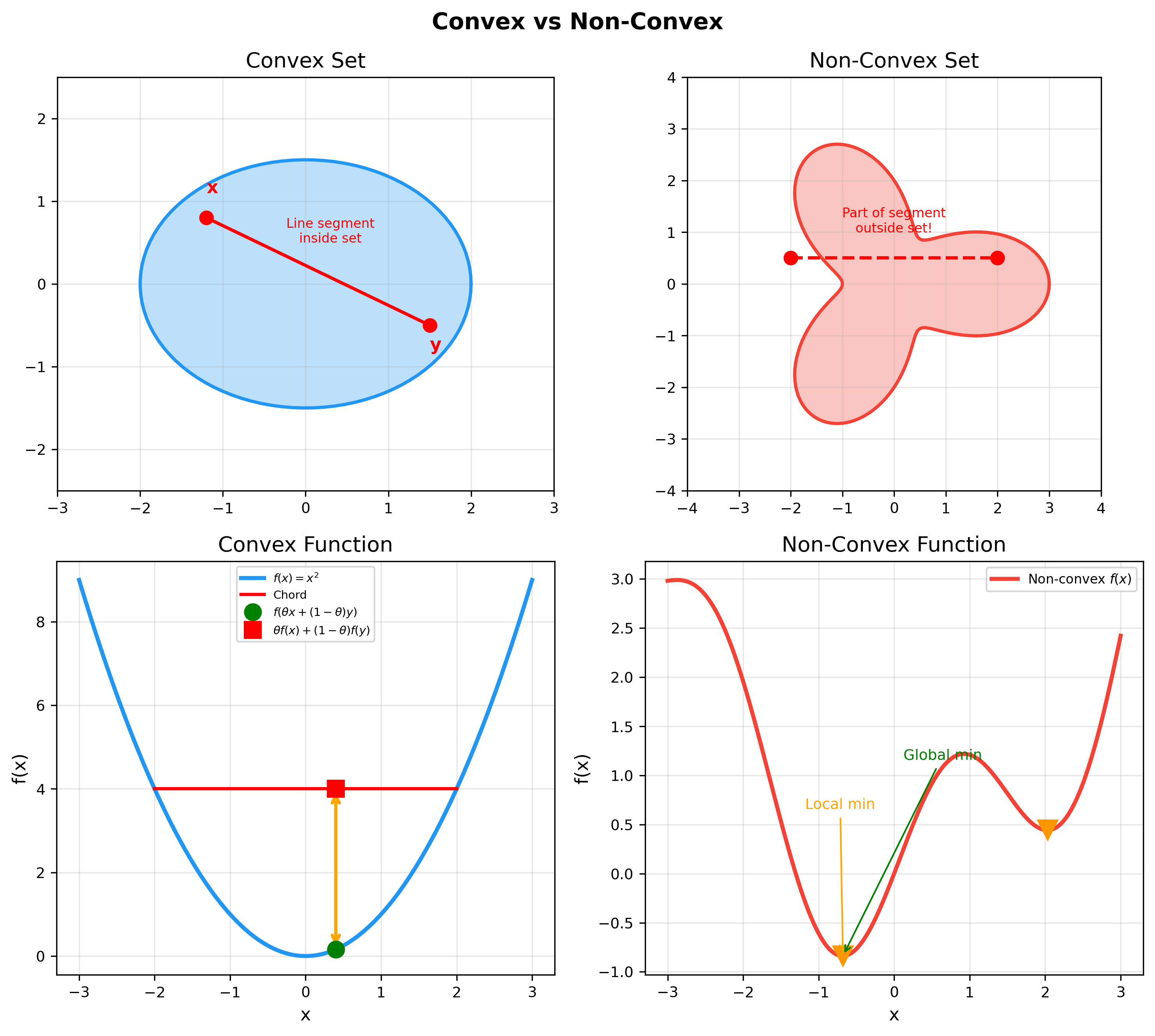
This definition states that the line segment connecting any two points in a convex set is entirely contained within the set. Geometrically, convex sets have no "indentations."

Convex Optimization Fundamentals

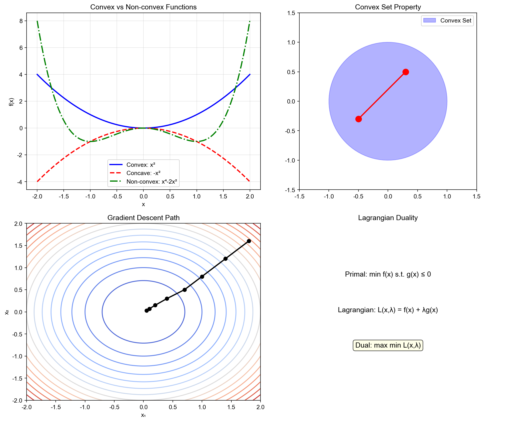
The following figure contrasts convex and non-convex sets/functions — convexity guarantees that local optima are global optima, which is the core value of convex optimization in machine learning:

Convex vs Non-Convex

Example 1 (Common Convex Sets):

1. Hyperplane:, where

2. Halfspace:

3. Norm ball:, for any norm

4. Ellipsoid:, where(positive definite)

Proof that hyperplane is convex: Let, meaningand. For any:

Therefore.

Theorem 1 (Intersection of Convex Sets): Ifis a family of convex sets, then is also convex.

Proof: Let , meaning for all . Since each is convex, for any:

Therefore.

This property is crucial: it means we can describe complex convex sets through the intersection of finitely many linear constraints (halfspaces).

Definition and Characterization of Convex Functions

Definition 2 (Convex Function): A function is convex if its domainis a convex set, and for any and any:

Geometric interpretation: the line segment between any two points on the function's graph lies above the function's graph.

Definition 3 (Strictly Convex Function): For any and, the inequality holds strictly:

Definition 4 (Strongly Convex Function): Function is -strongly convex () if is convex. Equivalently:

Strong convexity is a stronger condition than convexity, guaranteeing "strict quadratic growth."

Theorem 2 (First-Order Condition): A differentiable function is convex if and only if for any :

This shows that the first-order Taylor expansion of a convex function is a global lower bound (tangent lines always lie below the function).

Proof (Sufficiency): Assume the first-order condition holds. For anyand, let. By the first-order condition:

Multiply the first inequality by, the second by, and add:

Proof (Necessity): Assume is convex. For any and :

Rearranging and dividing by :

Taking , the left side converges to the directional derivative:

Theorem 3 (Second-Order Condition): A twice-differentiable function is convex if and only if its Hessian matrix is positive semidefinite everywhere:

If (positive definite), then is strictly convex.

Proof sketch: Use Taylor expansion. For a convex function, the second-order remainder must be non-negative:

By the first-order condition, , therefore:

This holds for all , which is equivalent to.

Example 2 (Common Convex Functions):

1. Affine function:(both convex and concave)

2. Exponential function:

3. Power function:, whenor()

4. Negative entropy:()

5. Norm:, for any norm

Jensen's Inequality: Core Property of Convex Functions

Theorem 4 (Jensen's Inequality): If is a convex function and is a random variable withexisting, then:

If is strictly convex and is not constant, the inequality is strict.

Proof (Discrete case): Lettake valueswith probabilities(satisfying). Use mathematical induction:

-: This is the definition of convex function - Assume it holds for. Forpoints:

Jensen's inequality is foundational for many inequalities in information theory, statistics, and machine learning. For instance, it directly implies the non-negativity of KL divergence.

Subgradients and Non-smooth Optimization

Definition of Subgradients

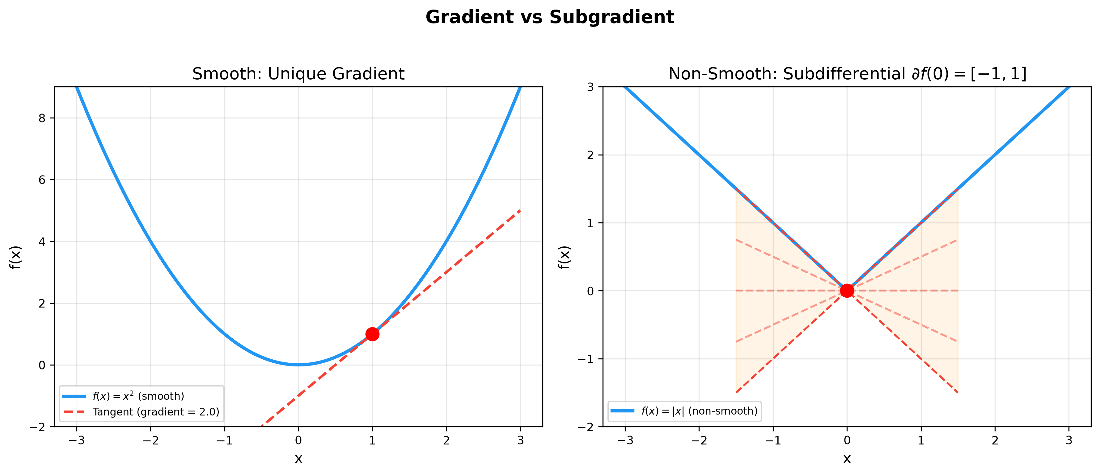
Convex functions may not be differentiable (e.g.,at), but we can still define a "generalized gradient."

Definition 5 (Subgradient): A vector is a subgradient of function at point if for all :

Geometric meaning: it defines a "supporting hyperplane" passing through point, which never lies above the function.

The figure below contrasts the gradient of smooth functions with subgradients of non-smooth functions — at non-differentiable points, the subdifferential is an interval, making non-smooth optimization possible:

Gradient vs Subgradient

Definition 6 (Subdifferential): The set of all subgradients at pointis called the subdifferential, denoted:

Theorem 5 (Properties of Subdifferential):

1. Ifis differentiable at, then(singleton set) 2.is a closed convex set 3.is an optimal solution if and only if Proof of property 3:

• Sufficiency: If, then for all:
• Necessity: Ifis optimal, thenfor all, sosatisfies the subgradient condition

Example 3 (Computing Subdifferentials):

1. Absolute value function:$$f(x) =

2. L1 norm:$$f(x) = {g : g_i = (x_i) x_i , |g_i| x_i = 0}

3. Indicator function(is a convex set):

This is called the normal cone ofat.

Subgradient Method

For non-differentiable convex functions, we can use subgradients instead of gradients for optimization.

Algorithm 1 (Subgradient Descent):

Initialize: x^(0)
for k = 0, 1, 2, ... do
    Choose g^(k) ∈ ∂ f(x^(k))
    x^(k+1) = x^(k) - α_k g^(k)
end for

whereis the step size.

Theorem 6 (Convergence of Subgradient Method): Assumeis a convex function withfor alland all. If the step size satisfies:

then.

Common step size choices include.

Proof sketch: Define. Using the subgradient condition and step size update:

Expanding and taking expectations establishes a recurrence relation, ultimately yielding.

First-Order Optimization Algorithms

Gradient Descent

Gradient descent is the most fundamental optimization algorithm, iteratively updating parameters in the direction of negative gradient.

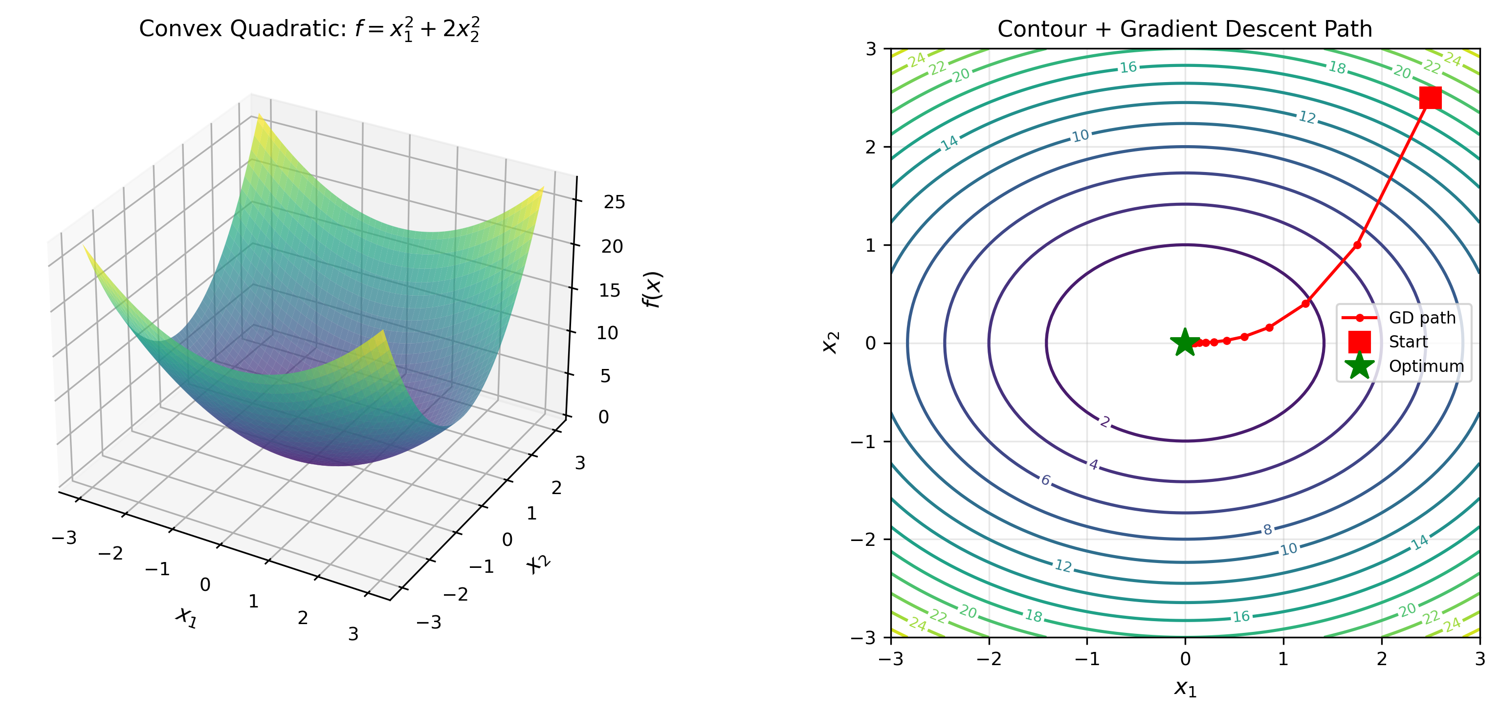
The animation below shows the gradient descent trajectory on 2D convex function contours — each step moves along the negative gradient direction, progressively approaching the optimum:

Gradient Descent Animation

Algorithm 2 (Gradient Descent):

Initialize: x^(0)
for k = 0, 1, 2, ... do
    x^(k+1) = x^(k) - α_k ∇ f(x^(k))
end for

Theorem 7 (Convergence of Gradient Descent - Convex and Smooth Case): Assumeis convex with-Lipschitz continuous gradient:

Using fixed step size, gradient descent satisfies:

This is a convergence rate of.

Proof:-smoothness is equivalent to:

Taking:

Using the first-order condition from convexity:

Combined with the recurrence for, we can derive the final result.

Theorem 8 (Strongly Convex Case): Ifis-strongly convex (i.e.,), gradient descent converges at a linear rate:

The convergence rate depends on the condition number.

Momentum and Nesterov Acceleration

Standard gradient descent converges slowly on "canyon" terrain (high curvature in one direction, low in another). Momentum methods accelerate by accumulating historical gradients.

Algorithm 3 (Momentum Gradient Descent):

Initialize: x^(0), v^(0) = 0
for k = 0, 1, 2, ... do
    v^(k+1) = β v^(k) - α ∇ f(x^(k))
    x^(k+1) = x^(k) + v^(k+1)
end for

whereis the momentum coefficient.

Nesterov Accelerated Gradient (NAG) makes a clever improvement: first "predict" the next position using momentum, then compute gradient at the predicted position:

Algorithm 4 (Nesterov Acceleration):

Initialize: x^(0), y^(0) = x^(0)
for k = 0, 1, 2, ... do
    x^(k+1) = y^(k) - α ∇ f(y^(k))
    y^(k+1) = x^(k+1) + β_k(x^(k+1) - x^(k))
end for

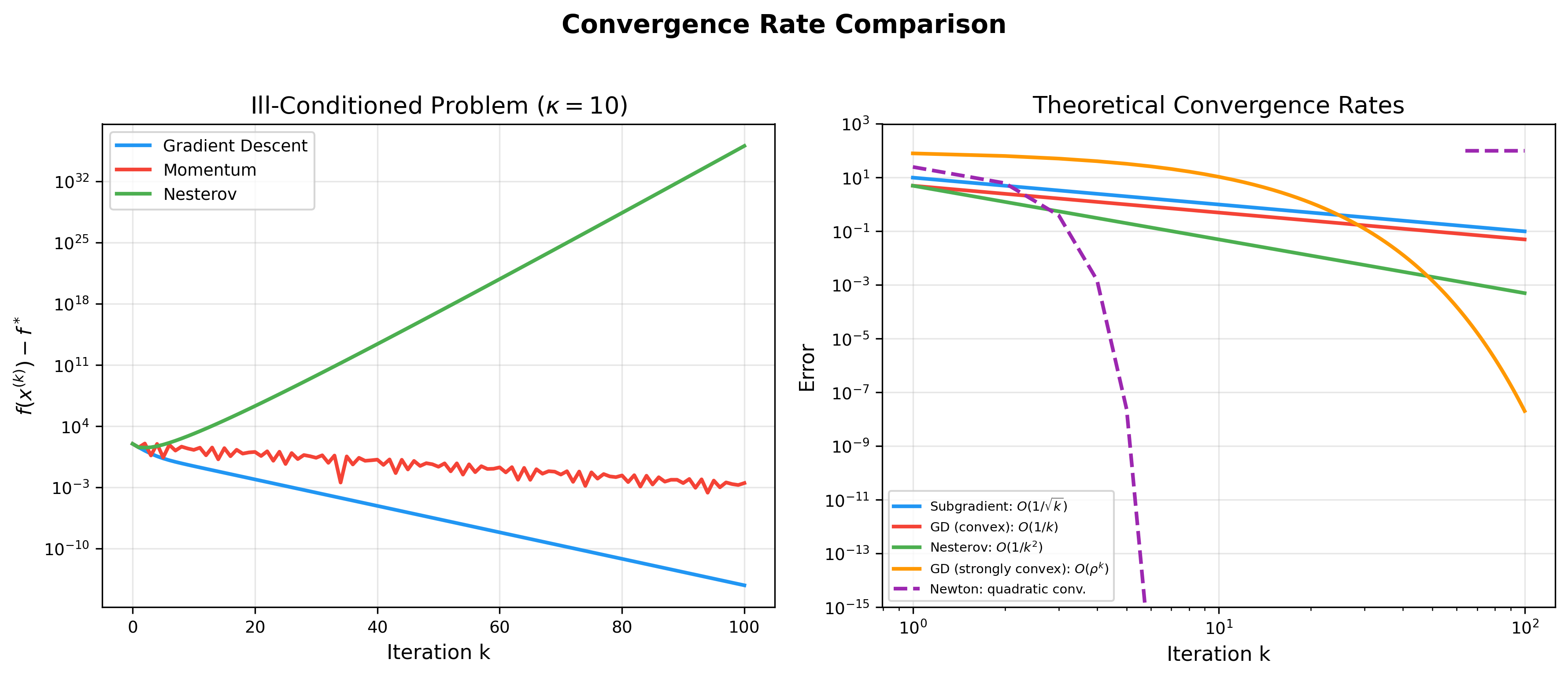
Theorem 9 (Nesterov Acceleration Convergence): For-smooth convex functions, Nesterov accelerated gradient method satisfies:

This is a convergence rate of , much faster than standard gradient descent's . This is theoretically the optimal rate for first-order methods in convex optimization.

The figure below compares convergence rates of various optimization algorithms — from subgradient method's to Newton's quadratic convergence:

Convergence Rate Comparison

Optimization Landscape

Adaptive Learning Rate Algorithms

Algorithms like AdaGrad, RMSProp, and Adam automatically adjust learning rates for each parameter based on historical gradients.

Algorithm 5 (Adam):

Initialize: x^(0), m^(0) = 0, v^(0) = 0
for k = 0, 1, 2, ... do
    g^(k) = ∇ f(x^(k))
    m^(k+1) = β_1 m^(k) + (1-β_1) g^(k)              // First moment estimate
    v^(k+1) = β_2 v^(k) + (1-β_2) (g^(k))^2          // Second moment estimate
    m ̂^(k+1) = m^(k+1) / (1 - β_1^{k+1})              // Bias correction
    v ̂^(k+1) = v^(k+1) / (1 - β_2^{k+1})
    x^(k+1) = x^(k) - α m ̂^(k+1) / (√ v ̂^(k+1)} + ε)
end for

Typical parameters:.

Adam combines momentum (first moment) and adaptive learning rates (second moment), making it widely used in deep learning.

Second-Order Optimization Algorithms

Newton's Method

Newton's method uses second-order information (Hessian matrix) to construct a quadratic approximation, achieving faster convergence.

Derivation: At point, perform second-order Taylor expansion of:

Taking derivative with respect toand setting to zero:

Solving for the Newton direction:

Algorithm 6 (Newton's Method):

Initialize: x^(0)
for k = 0, 1, 2, ... do
    Compute g^(k) = ∇ f(x^(k))
    Compute H^(k) = ∇² f(x^(k))
    Solve linear system: H^(k) Δ x^(k) = -g^(k)
    x^(k+1) = x^(k) + Δ x^(k)
end for

Theorem 10 (Quadratic Convergence of Newton's Method): Assumeis strongly convex andis Lipschitz continuous. If the initial pointis sufficiently close to the optimal solution, Newton's method converges quadratically:

Proof sketch: Use Taylor expansion and implicit function theorem. At optimal point,. Expandnear:

Newton iteration:

Substituting and simplifying yields quadratic convergence.

Disadvantages of Newton's method:

1. Each iteration requires computing and inverting anHessian matrix, computational complexity
2. Hessian may not be positive definite, causing search direction to not be a descent direction
3. Requires storingmatrix

Quasi-Newton Methods: BFGS Algorithm

Quasi-Newton methods approximate the Hessian matrixwith a matrix, avoiding direct Hessian computation and storage.

Quasi-Newton Condition (Secant Condition): We wantto satisfy:

Let,, then:

This mimics a property satisfied by the true Hessian (curvature information along the search direction).

BFGS Update Formula: The BFGS (Broyden-Fletcher-Goldfarb-Shanno) algorithm uses the following update:

Or update the inverse matrix(Sherman-Morrison-Woodbury formula):

where.

Algorithm 7 (BFGS):

Initialize: x^(0), H^(0) = I
for k = 0, 1, 2, ... do
    Compute g^(k) = ∇ f(x^(k))
    d^(k) = -H^(k) g^(k)
    Line search: choose α_k such that f(x^(k) + α_k d^(k)) is small enough
    x^(k+1) = x^(k) + α_k d^(k)
    s_k = x^(k+1) - x^(k)
    y_k = ∇ f(x^(k+1)) - ∇ f(x^(k))
    Update H^(k+1) using formula above
end for

Theorem 11 (Superlinear Convergence of BFGS): For strongly convex functions, if line search satisfies Wolfe conditions, BFGS converges superlinearly:

BFGS is one of the most successful quasi-Newton algorithms in practice, widely applied to small and medium-scale optimization problems.

L-BFGS (Limited-memory BFGS): For large-scale problems, storingis still infeasible. L-BFGS only stores the most recentiterations'pairs (typically), computingthrough recursive formulas.

Constrained Optimization and Duality Theory

Lagrangian Duality

Consider a general constrained optimization problem:

Lagrangian Function: Introduce Lagrange multipliers:

Definition 7 (Lagrangian Dual Function):

where.

Theorem 12 (Weak Duality): For any:

whereis the optimal value of the primal problem.

Proof: Letbe any feasible solution of the primal problem. Thenand. Since:

Therefore:

Sinceholds for all feasible solutions, we have.

Dual Problem:

Let the optimal value of the dual problem be. Weak duality tells us.

Definition 8 (Duality Gap):is called the duality gap. If, strong duality holds.

Theorem 13 (Slater's Condition): If the primal problem is a convex optimization problem (are convex functions,are affine functions), and there exists a strictly feasible point (i.e., there existssuch thatfor all,for all), then strong duality holds.

This condition guarantees zero duality gap, allowing us to solve the primal problem through the dual problem.

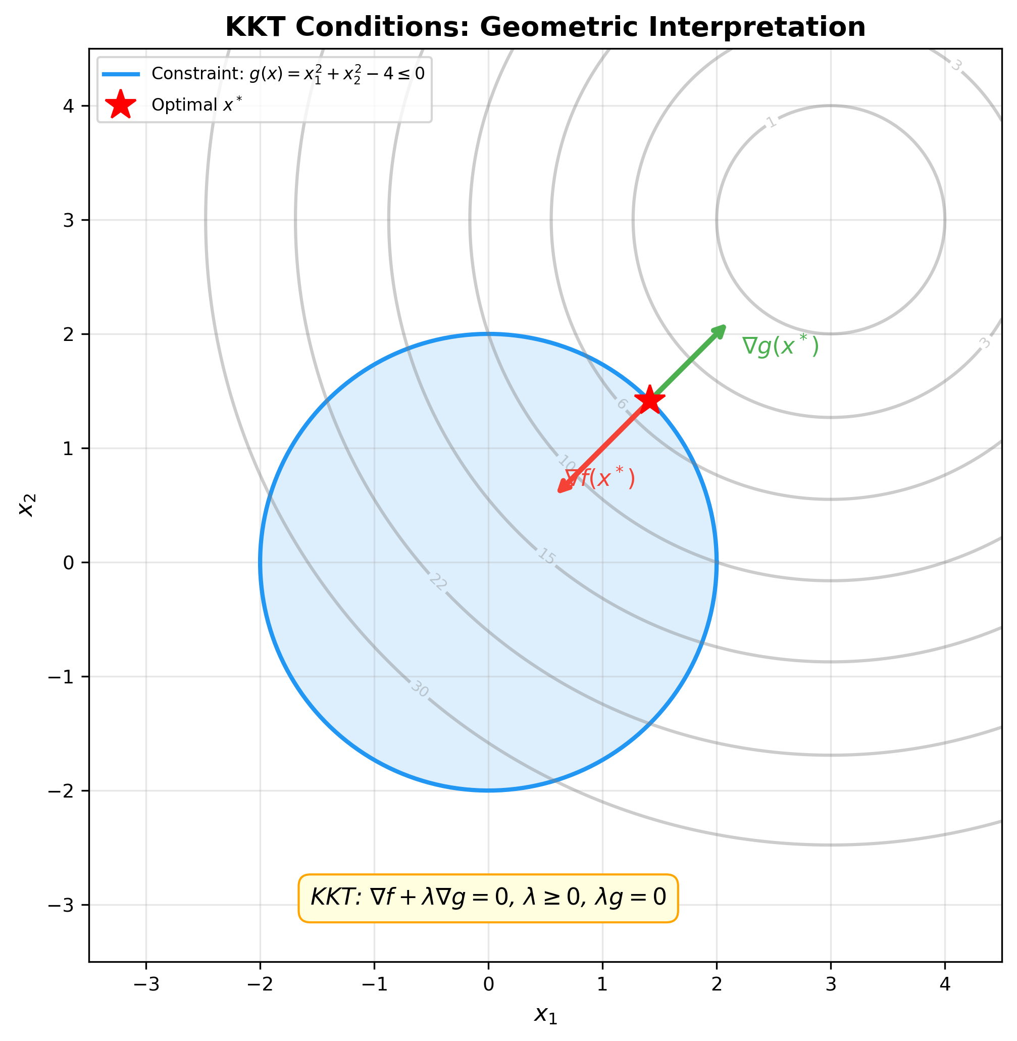
KKT Conditions: Necessary and Sufficient Conditions for Optimality

Theorem 14 (KKT Conditions): Assumeare differentiable. Ifare optimal solutions of the primal and dual problems respectively, and strong duality holds, they satisfy the Karush-Kuhn-Tucker (KKT) conditions:

1. Primal feasibility:

2. Dual feasibility:

3. Complementary slackness:

4. Stationarity:

The figure below shows the geometric interpretation of KKT conditions — at the optimum, the objective gradient and constraint gradient must be anti-parallel, and complementary slackness ensures Lagrange multipliers are nonzero only when constraints are active:

KKT Conditions

Theorem 15: If the primal problem is convex and satisfies Slater's condition, KKT conditions are necessary and sufficient for optimality.

Proof sketch (Complementary slackness): Sinceis the minimizer ofwith respect to, and strong duality holds:

The last inequality usesand. Therefore all inequalities are equalities, in particular:

Sinceand, this is only possible whenfor all.

Example 4 (KKT Conditions in SVM): SVM primal problem:

KKT conditions yield:

Complementary slackness shows: only points on the margin (support vectors) have.

ADMM Algorithm

Alternating Direction Method of Multipliers (ADMM) is a powerful distributed optimization algorithm, particularly suited for solving convex optimization problems with separable structure.

Problem Formulation

Consider the following problem:

whereare convex functions,are matrices,is a vector.

Augmented Lagrangian Function:

whereis the dual variable,is the penalty parameter.

ADMM Algorithm Steps

Algorithm 8 (ADMM):

Initialize: x^(0), z^(0), y^(0)
for k = 0, 1, 2, ... do
    x^(k+1) = argmin_x L_ρ(x, z^(k), y^(k))
    z^(k+1) = argmin_z L_ρ(x^(k+1), z, y^(k))
    y^(k+1) = y^(k) + ρ(Ax^(k+1) + Bz^(k+1) - c)
end for

Algorithm explanation:

1. -update: Fixand, minimize augmented Lagrangian with respect to
2. -update: Fixand, minimize with respect to
3. -update: Gradient ascent on dual variable

ADMM's cleverness: even if joint optimization ofis difficult, optimizingandseparately may be simple (closed-form solutions or efficient algorithms).

Convergence Analysis

Theorem 16 (ADMM Convergence): Assumeare closed convex functions and the problem has a solution. Then the sequencegenerated by ADMM satisfies:

1. Residual convergence:

2. Objective convergence:

3. Dual variable convergence: Proof sketch: Construct a Lyapunov function to prove sequence convergence. Define:

We can prove, thusdecreases monotonically.

Application Example: Lasso Regression

Lasso problem:

Rewrite in ADMM form:

Augmented Lagrangian function:

ADMM updates:

1. -update:

This is a ridge regression problem with closed-form solution.

2. -update:

where is the soft-thresholding operator:

3. -update:

This algorithm is very efficient and easily distributed.

Implementation Code

Below is a complete implementation of gradient descent, Newton's method, BFGS, and ADMM.

import numpy as np
from scipy.linalg import cho_factor, cho_solve
from typing import Callable, Tuple, Optional

class ConvexOptimizer:
    """Unified interface for convex optimization algorithms"""
    
    def __init__(self, 
                 f: Callable[[np.ndarray], float],
                 grad_f: Callable[[np.ndarray], np.ndarray],
                 hess_f: Optional[Callable[[np.ndarray], np.ndarray]] = None):
        """
        Parameters:
            f: Objective function
            grad_f: Gradient function
            hess_f: Hessian matrix function (optional, for second-order methods)
        """
        self.f = f
        self.grad_f = grad_f
        self.hess_f = hess_f
        self.history = {'x': [], 'f': [], 'grad_norm': []}
    
    def gradient_descent(self, 
                        x0: np.ndarray, 
                        alpha: float = 0.01,
                        max_iter: int = 1000,
                        tol: float = 1e-6) -> np.ndarray:
        """
        Gradient descent method
        
        Parameters:
            x0: Initial point
            alpha: Learning rate
            max_iter: Maximum iterations
            tol: Convergence tolerance
        """
        x = x0.copy()
        self.history = {'x': [x.copy()], 'f': [self.f(x)], 'grad_norm': []}
        
        for k in range(max_iter):
            grad = self.grad_f(x)
            grad_norm = np.linalg.norm(grad)
            self.history['grad_norm'].append(grad_norm)
            
            if grad_norm < tol:
                print(f"Gradient descent converged at iteration {k}")
                break
            
            # Gradient descent update
            x = x - alpha * grad
            
            self.history['x'].append(x.copy())
            self.history['f'].append(self.f(x))
        
        return x
    
    def gradient_descent_backtracking(self,
                                     x0: np.ndarray,
                                     alpha: float = 1.0,
                                     beta: float = 0.5,
                                     sigma: float = 0.1,
                                     max_iter: int = 1000,
                                     tol: float = 1e-6) -> np.ndarray:
        """
        Gradient descent with backtracking line search
        
        Parameters:
            x0: Initial point
            alpha: Initial step size
            beta: Step size reduction factor
            sigma: Armijo condition parameter
        """
        x = x0.copy()
        self.history = {'x': [x.copy()], 'f': [self.f(x)], 'grad_norm': []}
        
        for k in range(max_iter):
            grad = self.grad_f(x)
            grad_norm = np.linalg.norm(grad)
            self.history['grad_norm'].append(grad_norm)
            
            if grad_norm < tol:
                print(f"Gradient descent (backtracking) converged at iteration {k}")
                break
            
            # Backtracking line search
            t = alpha
            fx = self.f(x)
            while self.f(x - t * grad) > fx - sigma * t * grad_norm**2:
                t *= beta
            
            x = x - t * grad
            
            self.history['x'].append(x.copy())
            self.history['f'].append(self.f(x))
        
        return x
    
    def newton_method(self,
                     x0: np.ndarray,
                     max_iter: int = 100,
                     tol: float = 1e-6) -> np.ndarray:
        """
        Newton's method
        
        Requires: hess_f must be provided
        """
        if self.hess_f is None:
            raise ValueError("Newton's method requires Hessian function")
        
        x = x0.copy()
        self.history = {'x': [x.copy()], 'f': [self.f(x)], 'grad_norm': []}
        
        for k in range(max_iter):
            grad = self.grad_f(x)
            hess = self.hess_f(x)
            grad_norm = np.linalg.norm(grad)
            self.history['grad_norm'].append(grad_norm)
            
            if grad_norm < tol:
                print(f"Newton's method converged at iteration {k}")
                break
            
            # Solve linear system: H * delta = -grad
            try:
                delta = np.linalg.solve(hess, -grad)
            except np.linalg.LinAlgError:
                print("Hessian not invertible, switching to gradient descent")
                delta = -grad
            
            x = x + delta
            
            self.history['x'].append(x.copy())
            self.history['f'].append(self.f(x))
        
        return x
    
    def bfgs(self,
            x0: np.ndarray,
            max_iter: int = 1000,
            tol: float = 1e-6) -> np.ndarray:
        """
        BFGS quasi-Newton method
        """
        n = len(x0)
        x = x0.copy()
        H = np.eye(n)  # Initialize inverse Hessian approximation as identity
        
        self.history = {'x': [x.copy()], 'f': [self.f(x)], 'grad_norm': []}
        grad = self.grad_f(x)
        
        for k in range(max_iter):
            grad_norm = np.linalg.norm(grad)
            self.history['grad_norm'].append(grad_norm)
            
            if grad_norm < tol:
                print(f"BFGS converged at iteration {k}")
                break
            
            # Compute search direction
            d = -H @ grad
            
            # Backtracking line search
            alpha = 1.0
            beta = 0.5
            sigma = 0.1
            fx = self.f(x)
            while self.f(x + alpha * d) > fx + sigma * alpha * grad @ d:
                alpha *= beta
            
            # Update
            x_new = x + alpha * d
            grad_new = self.grad_f(x_new)
            
            # Compute s_k and y_k
            s = x_new - x
            y = grad_new - grad
            
            # BFGS update of inverse Hessian approximation
            rho = 1.0 / (y @ s)
            if rho > 0:  # Ensure positive definiteness
                I = np.eye(n)
                H = (I - rho * np.outer(s, y)) @ H @ (I - rho * np.outer(y, s)) + rho * np.outer(s, s)
            
            x = x_new
            grad = grad_new
            
            self.history['x'].append(x.copy())
            self.history['f'].append(self.f(x))
        
        return x
    
    def momentum_gd(self,
                   x0: np.ndarray,
                   alpha: float = 0.01,
                   beta: float = 0.9,
                   max_iter: int = 1000,
                   tol: float = 1e-6) -> np.ndarray:
        """
        Momentum gradient descent
        
        Parameters:
            beta: Momentum coefficient
        """
        x = x0.copy()
        v = np.zeros_like(x)
        self.history = {'x': [x.copy()], 'f': [self.f(x)], 'grad_norm': []}
        
        for k in range(max_iter):
            grad = self.grad_f(x)
            grad_norm = np.linalg.norm(grad)
            self.history['grad_norm'].append(grad_norm)
            
            if grad_norm < tol:
                print(f"Momentum gradient descent converged at iteration {k}")
                break
            
            # Momentum update
            v = beta * v - alpha * grad
            x = x + v
            
            self.history['x'].append(x.copy())
            self.history['f'].append(self.f(x))
        
        return x
    
    def nesterov_accelerated_gd(self,
                               x0: np.ndarray,
                               alpha: float = 0.01,
                               max_iter: int = 1000,
                               tol: float = 1e-6) -> np.ndarray:
        """
        Nesterov accelerated gradient method
        """
        x = x0.copy()
        y = x.copy()
        x_old = x.copy()
        
        self.history = {'x': [x.copy()], 'f': [self.f(x)], 'grad_norm': []}
        
        for k in range(max_iter):
            grad = self.grad_f(y)
            grad_norm = np.linalg.norm(grad)
            self.history['grad_norm'].append(grad_norm)
            
            if grad_norm < tol:
                print(f"Nesterov acceleration converged at iteration {k}")
                break
            
            # Nesterov update
            x_new = y - alpha * grad
            beta_k = k / (k + 3)  # Dynamic momentum coefficient
            y = x_new + beta_k * (x_new - x)
            
            x = x_new
            
            self.history['x'].append(x.copy())
            self.history['f'].append(self.f(x))
        
        return x


class ADMMSolver:
    """ADMM algorithm solver"""
    
    def __init__(self, rho: float = 1.0):
        """
        Parameters:
            rho: Augmented Lagrangian parameter
        """
        self.rho = rho
        self.history = {'primal_residual': [], 'dual_residual': [], 'objective': []}
    
    def solve_lasso(self,
                   X: np.ndarray,
                   y: np.ndarray,
                   lambda_: float,
                   max_iter: int = 1000,
                   tol: float = 1e-4) -> Tuple[np.ndarray, np.ndarray]:
        """
        Solve Lasso problem using ADMM:
        min (1/2)||y - X β||^2 + λ||β||_1
        
        Returns:
            beta: Regression coefficients
            z: Auxiliary variable
        """
        n, p = X.shape
        
        # Precompute
        XtX = X.T @ X
        Xty = X.T @ y
        L = cho_factor(XtX + self.rho * np.eye(p))
        
        # Initialize
        beta = np.zeros(p)
        z = np.zeros(p)
        u = np.zeros(p)
        
        for k in range(max_iter):
            # β update (ridge regression)
            beta = cho_solve(L, Xty + self.rho * (z - u))
            
            # z update (soft thresholding)
            z_old = z.copy()
            z = self._soft_threshold(beta + u, lambda_ / self.rho)
            
            # u update (dual variable)
            u = u + beta - z
            
            # Compute residuals
            primal_residual = np.linalg.norm(beta - z)
            dual_residual = self.rho * np.linalg.norm(z - z_old)
            
            self.history['primal_residual'].append(primal_residual)
            self.history['dual_residual'].append(dual_residual)
            self.history['objective'].append(
                0.5 * np.linalg.norm(y - X @ beta)**2 + lambda_ * np.linalg.norm(z, 1)
            )
            
            if primal_residual < tol and dual_residual < tol:
                print(f"ADMM converged at iteration {k}")
                break
        
        return beta, z
    
    @staticmethod
    def _soft_threshold(x: np.ndarray, kappa: float) -> np.ndarray:
        """Soft thresholding operator"""
        return np.sign(x) * np.maximum(np.abs(x) - kappa, 0)


# Example: Quadratic function optimization
def example_quadratic():
    """
    Minimize f(x) = (1/2) x^T Q x - b^T x
    where Q is positive definite
    """
    np.random.seed(42)
    n = 10
    A = np.random.randn(n, n)
    Q = A.T @ A + np.eye(n)  # Ensure positive definite
    b = np.random.randn(n)
    
    # True solution
    x_true = np.linalg.solve(Q, b)
    
    # Define functions
    f = lambda x: 0.5 * x @ Q @ x - b @ x
    grad_f = lambda x: Q @ x - b
    hess_f = lambda x: Q
    
    optimizer = ConvexOptimizer(f, grad_f, hess_f)
    
    x0 = np.random.randn(n)
    
    print("=" * 60)
    print("Testing Quadratic Function Optimization")
    print(f"True solution objective value: {f(x_true):.6f}")
    print()
    
    # Gradient descent
    x_gd = optimizer.gradient_descent_backtracking(x0.copy(), max_iter=1000)
    print(f"Gradient descent: f(x) = {f(x_gd):.6f}, ||x - x*|| = {np.linalg.norm(x_gd - x_true):.6e}")
    
    # Newton's method
    x_newton = optimizer.newton_method(x0.copy(), max_iter=100)
    print(f"Newton's method: f(x) = {f(x_newton):.6f}, ||x - x*|| = {np.linalg.norm(x_newton - x_true):.6e}")
    
    # BFGS
    x_bfgs = optimizer.bfgs(x0.copy(), max_iter=1000)
    print(f"BFGS: f(x) = {f(x_bfgs):.6f}, ||x - x*|| = {np.linalg.norm(x_bfgs - x_true):.6e}")
    
    # Momentum
    x_momentum = optimizer.momentum_gd(x0.copy(), alpha=0.01, max_iter=1000)
    print(f"Momentum: f(x) = {f(x_momentum):.6f}, ||x - x*|| = {np.linalg.norm(x_momentum - x_true):.6e}")
    
    # Nesterov
    x_nesterov = optimizer.nesterov_accelerated_gd(x0.copy(), alpha=0.01, max_iter=1000)
    print(f"Nesterov: f(x) = {f(x_nesterov):.6f}, ||x - x*|| = {np.linalg.norm(x_nesterov - x_true):.6e}")


def example_lasso():
    """Lasso regression example"""
    np.random.seed(42)
    n, p = 100, 50
    
    # Generate sparse true coefficients
    beta_true = np.zeros(p)
    beta_true[:10] = np.random.randn(10)
    
    # Generate data
    X = np.random.randn(n, p)
    y = X @ beta_true + 0.1 * np.random.randn(n)
    
    lambda_ = 0.1
    
    print("\n" + "=" * 60)
    print("Testing ADMM for Lasso")
    print(f"Data dimensions: n={n}, p={p}")
    print(f"True sparsity: {np.sum(beta_true != 0)}")
    print()
    
    solver = ADMMSolver(rho=1.0)
    beta_admm, z_admm = solver.solve_lasso(X, y, lambda_, max_iter=1000)
    
    print(f"ADMM sparsity: {np.sum(np.abs(z_admm) > 1e-4)}")
    print(f"Reconstruction error: {np.linalg.norm(beta_admm - beta_true):.6f}")
    print(f"Prediction MSE: {np.mean((y - X @ beta_admm)**2):.6f}")


if __name__ == "__main__":
    example_quadratic()
    example_lasso()

Code explanation:

1. ConvexOptimizer class: Implements multiple optimization algorithms
   • gradient_descent: Fixed step size gradient descent
   • gradient_descent_backtracking: Gradient descent with backtracking line search
   • newton_method: Newton's method
   • bfgs: BFGS quasi-Newton method
   • momentum_gd: Momentum gradient descent
   • nesterov_accelerated_gd: Nesterov acceleration
2. ADMMSolver class: Implements ADMM algorithm for Lasso
   • Uses Cholesky decomposition to accelerateupdate
   • Soft thresholding operator forupdate
   • Tracks primal and dual residuals
3. Examples:
   • Quadratic function optimization: Demonstrates convergence performance of different algorithms
   • Lasso regression: Demonstrates ADMM application in sparse optimization

In-Depth Q&A

Q1: Why is convex optimization so important? Isn't non-convex optimization more common?

A1: The importance of convex optimization manifests in three layers:

1. Theoretical level: Convex optimization is the only class of problems where we can completely characterize optimality conditions. KKT conditions provide necessary and sufficient conditions, which is impossible in non-convex cases.

2. Algorithmic level: Convex optimization has polynomial-time algorithms (like interior-point methods), with strict convergence guarantees. Gradient descent in convex cases guarantees convergence to global optimum, while in non-convex cases it only guarantees local optimum.

3. Application level: Many practical problems are inherently convex (linear regression, support vector machines, many statistical estimation problems). Even when the original problem is non-convex, convex relaxation techniques can provide useful approximate solutions and lower bounds.

For non-convex problems like deep learning, convex optimization theory still provides important intuition and tools. For instance, adaptive algorithms like Adam draw design inspiration from dual averaging methods in convex optimization.

Q2: What is the relationship between Jensen's inequality and the non-negativity of KL divergence?

A2: The non-negativity of KL divergence is a direct consequence of Jensen's inequality. KL divergence is defined as:

To prove, note thatis a convex function. By Jensen's inequality:

Equality holds if and only if(property of strictly convex functions).

This proof reveals the deep connection between information theory and convex optimization. KL divergence can be viewed as a "distance" in probability distribution space (though asymmetric), and Jensen's inequality guarantees this "distance" is always non-negative.

Q3: Why is Newton's method faster than gradient descent, but less commonly used in practice?

A3: This is a classic theory-practice trade-off:

Advantages of Newton's method: - Quadratic convergence: Error decreases quadratically per iteration, extremely fast near optimum - Adaptive step size: Automatically adjusts step size based on curvature, no parameter tuning needed - Affine invariance: Insensitive to coordinate transformations

Disadvantages of Newton's method: 1. Computational cost: Each iteration requiresto compute/invert Hessian. Forproblems, this is infeasible. 2. Storage cost: Need to storeHessian matrix,memory. 3. Non-positive definite issues: If Hessian is not positive definite, Newton direction may not be descent direction, requiring additional correction (like adding regularization). 4. Global convergence: Newton's method only has local quadratic convergence; may diverge far from optimum.

Practical solutions: - Small-scale problems (): Direct Newton or BFGS - Medium-scale (): L-BFGS, storing only recent iteration information - Large-scale (): First-order methods (SGD, Adam), or exploit structure (like block-diagonal Hessian approximations in deep learning) - Distributed ultra-large-scale: ADMM, exploiting separable structure

Q4: How is the BFGS update formula derived?

A4: BFGS update formula derivation is based on two principles:

Principle 1: Satisfy quasi-Newton condition (Secant equation)

Principle 2: Minimize(in some norm)

Specific derivation: Consider optimization problem

This is a constrained optimization problem. Construct Lagrangian and solve to get:

The first term "removes"'s information in direction, the second term "adds" new curvature information.

Symmetric rank-1 (SR1) formula is another choice:

But SR1 may not maintain positive definiteness, while BFGS guarantees positive definiteness when(naturally satisfied in convex functions).

Q5: Why can ADMM be implemented in a distributed manner?

A5: ADMM's distributed capability stems from its "divide and conquer" structure. Consider multi-agent collaborative optimization:

Each agent only knows its own. ADMM allows each agent to independently update, requiring only minimal information exchange with a central node.

Global consensus ADMM:

// Agent i's local update (parallel)
x_i^(k+1) = argmin_{x_i} [f_i(x_i) + y_i^(k)T x_i + (ρ/2)||x_i - z^(k)||^2]

// Central node's global update
z^(k+1) = (1/N) Σ_i x_i^(k+1)

// Dual variable update
y_i^(k+1) = y_i^(k) + ρ(x_i^(k+1) - z^(k+1))

Each iteration, agents only sendto center, center only broadcasts. Communication is, not.

This makes ADMM particularly suitable for: - Federated learning: Each client trains local model, server aggregates - Sensor networks: Distributed state estimation - Large-scale machine learning: Data distributed across multiple nodes

Q6: What is the practical significance of strong convexity? Why care about condition number?

A6: Strong convexity determines the optimization problem's "ill-conditioning" degree, directly affecting algorithm convergence speed.

Condition number(max curvature/min curvature) measures function's non-uniformity across directions:

-(perfect condition): Function is spherical, same curvature in all directions. Gradient descent converges in one step. -: Function is ellipsoidal, long axis 10× short axis. Gradient descent converges at rate. -(ill-conditioned): Function is extremely flat ellipsoid. Gradient descent converges at rate, requiring millions of iterations to significantly reduce error.

Example: Ridge regression condition number

Hessian matrix. Condition number:

Whenis very small,, can be large (multicollinearity). Increasingreduces condition number, improving numerical stability — an additional benefit of ridge regression.

Preconditioning techniques: For ill-conditioned problems, variable substitution can improve condition number. If, precondition variables with:

New problem's Hessian approaches identity matrix, condition number approaches 1. This is the idea behind Preconditioned Conjugate Gradient (PCG).

Q7: Why does subgradient method converge slower than gradient descent?

A7: This stems from information loss due to non-smoothness:

Gradient descent (smooth functions): - Gradient provides precise information about "steepest descent direction" - Step size can be precisely chosen based on Lipschitz constant - Convergence rate:(convex) or(strongly convex)

Subgradient method (non-smooth functions): - Subgradient is only a "supporting direction," not necessarily descent direction - Function value may increase in some iterations! - Must use decreasing step size (like) - Convergence rate: Intuitive explanation: Considernear. True optimal solution is, but subgradient arbitrarily chosen in, may point in wrong direction. Smooth function gradients gradually decrease approaching optimal solution, naturally "braking"; subgradients remain bounded at optimal solution, lacking this adaptivity.

Improvement methods: 1. Proximal gradient method: For, whereis smooth,is non-smooth (like L1 norm), can achieve. 2. Smoothing techniques: Approximate non-smooth functions with smooth ones, e.g., useto approximate. 3. Bundle methods: Accumulate multiple subgradient information to construct better descent directions.

Q8: What are the practical applications of Lagrangian duality in machine learning?

A8: Duality theory has multiple key applications in machine learning:

1. Support Vector Machines (SVM) - Primal problem: Optimize in high-dimensional or even infinite-dimensional space (when using kernels) - Dual problem: Only depends on inner productsbetween samples, can use kernel trick - KKT conditions yield sparsity: Most, only support vectors have 2. Theoretical Analysis of Neural Networks - Dual norms used to analyze generalization: Spectral norm, Frobenius norm of weight matrices, etc. - Lagrangian relaxation for neural network verification (proving property holds on all inputs)

3. Distributed Optimization - Primal problem may have complex global constraints - Dual problem can decompose into multiple independent subproblems, suitable for parallel computation - This is the theoretical basis of ADMM

4. Model Compression and Pruning - Sparse optimization (L0 norm minimization) is non-convex - L1 norm convex relaxation and its dual provide computable approximations

5. Generative Adversarial Networks (GAN) - GAN training is a min-max problem (saddle point problem) - Duality theory helps understand GAN convergence and equilibrium points - Wasserstein GAN directly optimizes dual form

Q9: How to choose optimization algorithms in practice?

A9: Choosing optimization algorithms requires considering multiple factors:

Factor	Recommended Algorithm
Problem Scale
Small-scale ()	BFGS, Newton's method
Medium-scale ()	L-BFGS, Conjugate Gradient
Large-scale ()	SGD, Adam, AdaGrad
Function Properties
Smooth convex	Gradient descent, Nesterov acceleration
Non-smooth convex	Subgradient method, Proximal gradient
Strongly convex	Newton, BFGS (fast convergence)
Ill-conditioned (large condition number)	Preconditioning, Adaptive algorithms
Constraints
Unconstrained	Above first/second-order methods
Simple constraints (e.g.,)	Projected gradient, Frank-Wolfe
Complex constraints	Augmented Lagrangian, Interior-point
Separable structure	ADMM
Computational Resources
Gradient easy, Hessian hard	First-order methods, Quasi-Newton
Distributed environment	ADMM, Distributed SGD
Online learning (streaming data)	SGD, Online gradient descent

Practical recommendations: 1. Start simple: Begin with gradient descent + line search, ensure correct implementation 2. Monitor convergence: Plot objective value, gradient norm curves 3. Tuning strategy: Learning rate is most critical parameter, use learning rate decay or adaptive algorithms 4. Combined use: First use first-order methods to quickly approach optimum, then second-order methods for fine optimization

Q10: What insights does convex optimization theory provide for deep learning (non-convex optimization)?

A10: Although deep learning loss functions are non-convex, convex optimization theory still provides important guidance:

1. Algorithm Design Inspiration - Adam's design borrows from dual averaging and adaptive step sizes in convex optimization - Batch Normalization can be viewed as implicit preconditioning, improving optimization condition number - Residual connections make optimization surface more convex-like (reducing gradient vanishing)

2. Local Convexity Analysis - Though globally non-convex, loss functions are approximately strongly convex near local minima - Can analyze algorithm behavior locally using convex optimization convergence rates - This explains why gradient descent converges quickly approaching minima

3. Generalization Theory - Regularization theory from convex optimization (L1, L2) directly applies to deep learning - Tools like PAC-Bayes bounds, Rademacher complexity all based on convex analysis

4. Loss Function Design - Understanding why cross-entropy is better than mean squared error for classification (from log-barrier functions in convex optimization) - Hinge loss, smoothed hinge loss design comes from convex optimization

5. Theoretical Guarantees in Degenerate Cases - Some deep learning problems provably convex (like single hidden layer linear network's matrix factorization form) - Over-parameterization theory shows sufficiently wide networks' optimization surfaces are "near-convex" in some sense

6. Identifying Optimization Traps - Convex optimization tells us characteristics of saddle points, local minima - In non-convex cases, we can use similar analysis to understand why SGD escapes saddle points (noise helps cross barriers)

Latest Research Directions: - Implicit bias: What kind of solutions does gradient descent tend to find in non-convex problems? Answer involves convex analysis. - Neural Tangent Kernel (NTK) theory: Extremely wide networks' training dynamics can be approximated by linear (convex) models. - Landscape theory: Study geometric structure of non-convex loss surfaces, identify "easy to optimize" non-convex problem classes.

✏️ Exercises and Solutions

Exercise 1: Convexity Verification

Problem: Determine whether the following functions are convex and prove your conclusions: (a) () (b) () (c)

Solution:

1. always holds, so is convex.

2. , (), so is convex.

3. The Hessian is, with eigenvaluesand. The Hessian is not positive semidefinite, so is not convex.

Exercise 2: KKT Conditions

Problem: Solve the following constrained optimization problem:

Solution:

Standard form: .

KKT conditions: 1. Stationarity: 2. Dual feasibility: 3. Complementary slackness: 4. Primal feasibility:

From condition 1: .

If, then , violating .

Therefore, and complementary slackness requires , i.e., , giving.

Optimal solution: , .

Exercise 3: Gradient Descent Convergence

Problem: For (where is symmetric positive definite), prove that gradient descent with fixed step size converges when.

Solution:

GD update: .

Therefore .

Convergence requires spectral radius.

Eigenvalues of are. We needfor all , i.e., .

Since ( is positive definite), the condition becomes.

Optimal step sizegives fastest convergence with rate, whereis the condition number.

Exercise 4: Dual Problem Derivation

Problem: Derive the dual of linear program.

Solution:

Lagrangian with multipliers (for ) and (for ):

Dual function:

Dual problem (eliminating):

This is the classic LP dual form. Strong duality holds since LP satisfies Slater's condition.

Exercise 5: Jensen's Inequality Application

Problem: Use Jensen's inequality to prove the AM-GM inequality: for ,

Solution:

Since is convex (), by Jensen's inequality:

Taking negatives and using monotonicity of:

QED.

References

This chapter's derivations and theory are primarily based on the following classic literature:

1. Boyd, S., & Vandenberghe, L. (2004). Convex Optimization. Cambridge University Press. [Classic textbook, standard reference for convex optimization]

2. Nocedal, J., & Wright, S. J. (2006). Numerical Optimization (2nd ed.). Springer. [Authoritative textbook on numerical optimization, detailed algorithm descriptions]

3. Nesterov, Y. (2004). Introductory Lectures on Convex Optimization: A Basic Course. Springer. [Original literature on Nesterov acceleration]

4. Duchi, J., Hazan, E., & Singer, Y. (2011). Adaptive Subgradient Methods for Online Learning and Stochastic Optimization. Journal of Machine Learning Research, 12, 2121-2159. [AdaGrad algorithm]

5. Kingma, D. P., & Ba, J. (2015). Adam: A Method for Stochastic Optimization. ICLR. [Adam algorithm, most commonly used optimizer in deep learning]

6. Boyd, S., Parikh, N., Chu, E., Peleato, B., & Eckstein, J. (2011). Distributed Optimization and Statistical Learning via the Alternating Direction Method of Multipliers. Foundations and Trends in Machine Learning, 3(1), 1-122. [Authoritative ADMM survey]

7. Bottou, L., Curtis, F. E., & Nocedal, J. (2018). Optimization Methods for Large-Scale Machine Learning. SIAM Review, 60(2), 223-311. [Modern survey on large-scale machine learning optimization]

8. Bubeck, S. (2015). Convex Optimization: Algorithms and Complexity. Foundations and Trends in Machine Learning, 8(3-4), 231-357. [Theoretical analysis of convex optimization algorithm complexity]

9. Beck, A., & Teboulle, M. (2009). A Fast Iterative Shrinkage-Thresholding Algorithm for Linear Inverse Problems. SIAM Journal on Imaging Sciences, 2(1), 183-202. [FISTA algorithm, accelerated proximal gradient]

10. Rockafellar, R. T. (1970). Convex Analysis. Princeton University Press. [Mathematical foundations of convex analysis]

11. Shalev-Shwartz, S., & Ben-David, S. (2014). Understanding Machine Learning: From Theory to Algorithms. Cambridge University Press. [Optimization theory in machine learning]

12. Polyak, B. T. (1964). Some methods of speeding up the convergence of iteration methods. USSR Computational Mathematics and Mathematical Physics, 4(5), 1-17. [Original literature on momentum method]

---

Summary: Convex optimization theory is the mathematical cornerstone of machine learning. This chapter rigorously derives the core theory (Jensen's inequality, subgradients, KKT conditions) and main algorithms (gradient descent, Newton's method, BFGS, ADMM) of convex optimization, starting from the definitions of convex sets and convex functions. Understanding these theories not only helps us design better algorithms, but also provides important intuition and tools for analyzing non-convex optimization (like deep learning). In subsequent chapters, we will see how these optimization techniques apply to specific machine learning models.