In 1912, Fisher proposed the idea of Maximum Likelihood Estimation (MLE), fundamentally transforming statistics. His core insight was: The best estimate of parameters should maximize the probability of observed data. Behind this seemingly simple idea lies profound mathematical structure — from the axiomatic definition of probability spaces, to asymptotic properties of statistical inference, to philosophical disputes between Bayesian and frequentist schools.

The core of machine learning is uncertainty modeling. Linear regression assumes errors follow Gaussian distribution; logistic regression assumes labels follow Bernoulli distribution; Hidden Markov Models assume state transitions follow Markov chains. All these models are built on the solid foundation of probability theory. This chapter derives the mathematical theory of statistical inference starting from Kolmogorov axioms.

Probability Spaces and Measure Theory Foundations

Axiomatic Definition of Probability Spaces

Definition 1 (Probability Space): A probability space is a triplet, where:

Sample space: set of all possible outcomes
Event σ-algebra : collection of subsets of satisfying σ-algebra properties:
- If , then (closed under complement)
- If , then (closed under countable union)
Probability measure , satisfying Kolmogorov axioms:
- Non-negativity: ,
- Normalization:
- Countable additivity: If are disjoint, then

Why do we need σ-algebra?

In infinite sample spaces, not all subsets are measurable. For example, there exist non-measurable sets (Vitali sets) on real interval. The σ-algebra ensures we only consider "well-behaved" events, giving probability measures good mathematical properties.

Theorem 1 (Basic Properties of Probability):

If , then
(inclusion-exclusion)

Proof of property 1:

By countable additivity, let , then:

This holds if and only if . QED.

Conditional Probability and Independence

Definition 2 (Conditional Probability): Let , the conditional probability of event given event is defined as:

Theorem 2 (Multiplication Rule):

Theorem 3 (Law of Total Probability): Letbe a partition of (i.e., are disjoint and), then for any event :

Proof:

Since are disjoint, are also disjoint. By countable additivity:

QED.

Theorem 4 (Bayes' Theorem): Let , then:

where the second equality uses law of total probability.

Meaning of Bayes' Theorem:

-: prior probability, belief aboutbefore observing data -: likelihood, probability of observinggiven -: posterior probability, updated belief aboutafter observing -: evidence, marginal probability of data

Bayes' theorem is the core of Bayesian statistics, providing mathematical framework for updating beliefs from data.

Definition 3 (Independence): Events and are independent if:

Equivalently, if , then .

Definition 4 (Conditional Independence): Events and are conditionally independent given event , denoted , if:

Note: Independence does not imply conditional independence, and conditional independence does not imply independence.

Counterexample: Consider flipping two coins:

-: first coin is heads -: second coin is heads -: exactly one coin is heads

Clearlyandare independent. But conditional on,andare not independent: if we know exactly one is heads and first is heads, then second must be tails.

Random Variables and Distributions

Definition 5 (Random Variable): A random variable is a measurable function from sample space to real numbers:

Measurability requires: for any Borel set , .

Definition 6 (Cumulative Distribution Function, CDF): The CDF of random variable is defined as:

Properties of CDF:

Monotone non-decreasing:
Right-continuous:
Limit properties: ,

Definition 7 (Probability Density Function, PDF): If there exists non-negative function such that:

then is called the probability density function of . In this case, is a continuous random variable.

Definition 8 (Probability Mass Function, PMF): For discrete random variable , its PMF is defined as:

Definition 9 (Joint Distribution): The joint CDF of random variablesis defined as:

Joint PDF (if exists):

Definition 10 (Marginal Distribution):

Definition 11 (Conditional Distribution):

Definition 12 (Independence of Random Variables): Random variables and are independent if:

Expectation, Variance, and Characteristic Functions

Definition and Properties of Expectation

Definition 13 (Expectation): The expectation of random variableis defined as:

Discrete:
Continuous:

Theorem 5 (Linearity of Expectation):

for any constants and random variables (even if not independent).

Proof (continuous case):

QED.

Theorem 6 (Law of Total Expectation):

Proof:

QED.

Variance and Covariance

Definition 14 (Variance):

Theorem 7 (Properties of Variance):

If and are independent, then Proof of property 2:

If and are independent, then , and the last term is 0. QED.

Definition 15 (Covariance):

Properties:

1.$(X, X) = (X)(X, Y) = (Y, X)(X + Y, Z) = (X, Z) + (Y, Z)XY(X, Y) = 0$(but converse not true)

Definition 16 (Correlation Coefficient):

Theorem 8 (Cauchy-Schwarz Inequality):

i.e., .

Proof: Consider any :

This is quadratic in , always non-negative, so discriminant:

QED.

Characteristic Functions

Definition 17 (Characteristic Function): The characteristic function of random variableis defined as:

Properties of characteristic functions:

(conjugate)
If , then
If and are independent, then

Theorem 9 (Uniqueness of Characteristic Function): Distribution is uniquely determined by characteristic function. I.e., if, thenandhave same distribution.

Theorem 10 (Moment Generating Property): If , then:

Proof:

Taking -th derivative with respect to :

Setting :

QED.

Common Probability Distributions

Discrete Distributions

1. Bernoulli Distribution

Definition:if:

Expectation and Variance:

Application: Binary classification, output distribution of logistic regression.

2. Binomial Distribution

Definition:represents number of successes inindependent Bernoulli trials:

Expectation and Variance:

Derivation of expectation:

Let, whereare i.i.d. By linearity of expectation:

Derivation of variance:

By independence additivity of variance:

3. Poisson Distribution

Definition: if:

Expectation and Variance:

Derivation of expectation:

Poisson's Theorem: When,, andfixed,.

Proof:

As :

So . QED.

Application: Counting rare events (e.g., website visits, radioactive decay).

Continuous Distributions

1. Uniform Distribution

Definition: if:

Expectation and Variance:

2. Exponential Distribution

Definition: if:

Expectation and Variance:

Memoryless property:

Proof:

QED.

Application: Waiting times, lifetime distributions, inter-arrival times in Poisson processes.

3. Gaussian Distribution (Normal)

Definition: if:

Expectation and Variance:

Standard Normal Distribution: , CDF denoted.

Standardization: If , then .

Multivariate Gaussian Distribution: , where , , positive definite:

Properties:

Invariance under linear transformation: If, then
Marginals are Gaussian: Ifjointly Gaussian, then marginalsandare Gaussian
Conditionals are Gaussian: Ifjointly Gaussian, thenandare Gaussian
Uncorrelated implies independent: For Gaussian random variables, Why is Gaussian distribution so important?
Central Limit Theorem: Sum of i.i.d. random variables tends to Gaussian
Maximum Entropy Principle: Among all distributions with given mean and variance, Gaussian has maximum entropy
Analytical tractability: Convolution and linear transformation of Gaussians are Gaussian
Ubiquity: Many natural phenomena approximately Gaussian (e.g., measurement errors)

4. Gamma Distribution

Definition:if:

whereis Gamma function.

Expectation and Variance:

Special cases:

-: Exponential distribution -: Chi-squared distribution

5. Beta Distribution

Definition: if:

Expectation and Variance:

Application: Conjugate prior in Bayesian inference (prior for Bernoulli/Binomial distribution).

Relationships Between Distributions

Theorem 11 (Relationship Between Gamma and Beta Functions):

Theorem 12 (Chi-squared Distribution): If independent, then:

Theorem 13 (t Distribution): If , , and , then:

where is t-distribution with degrees of freedom, PDF:

Theorem 14 (F Distribution): If , , and , then:

Common Probability Distributions

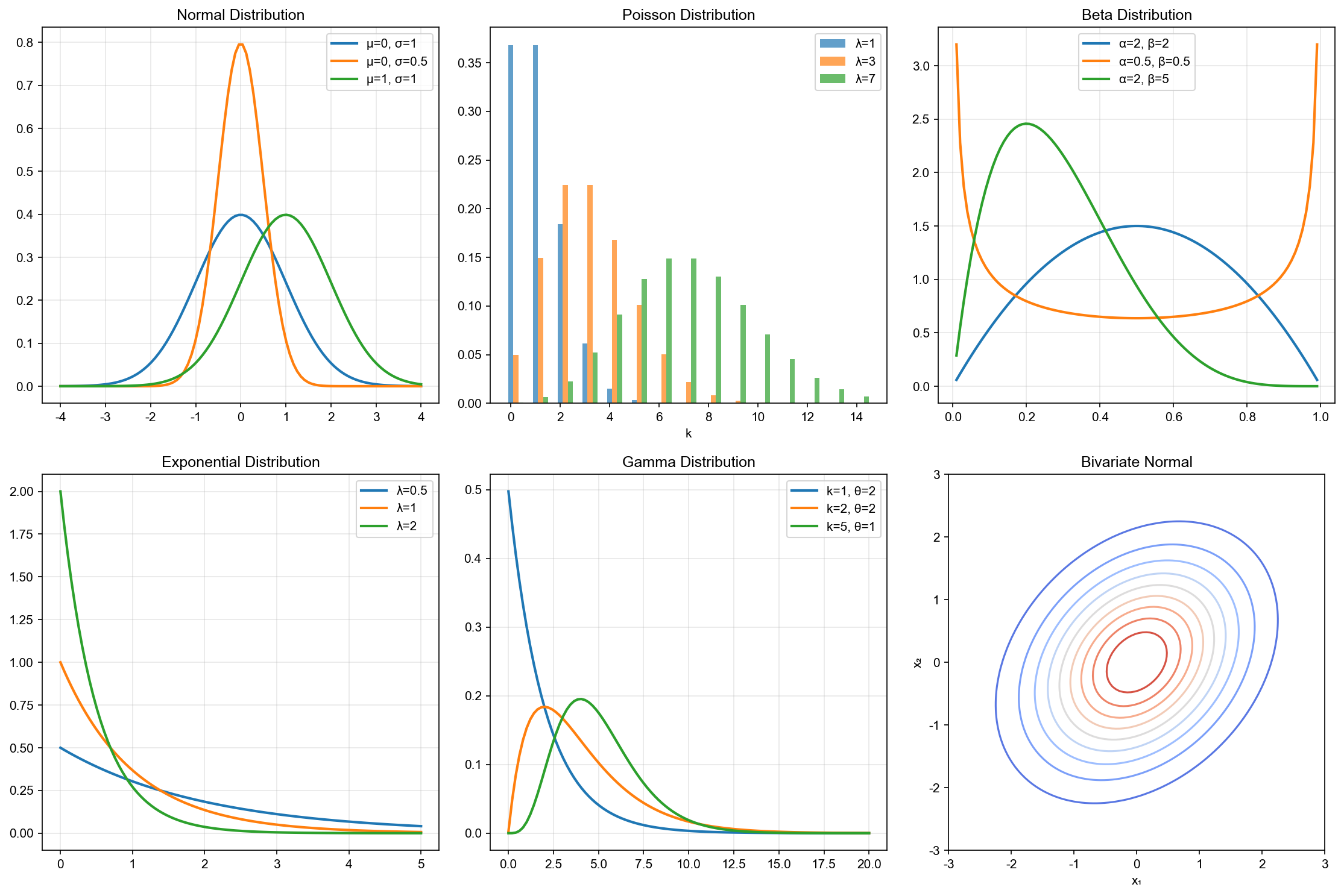
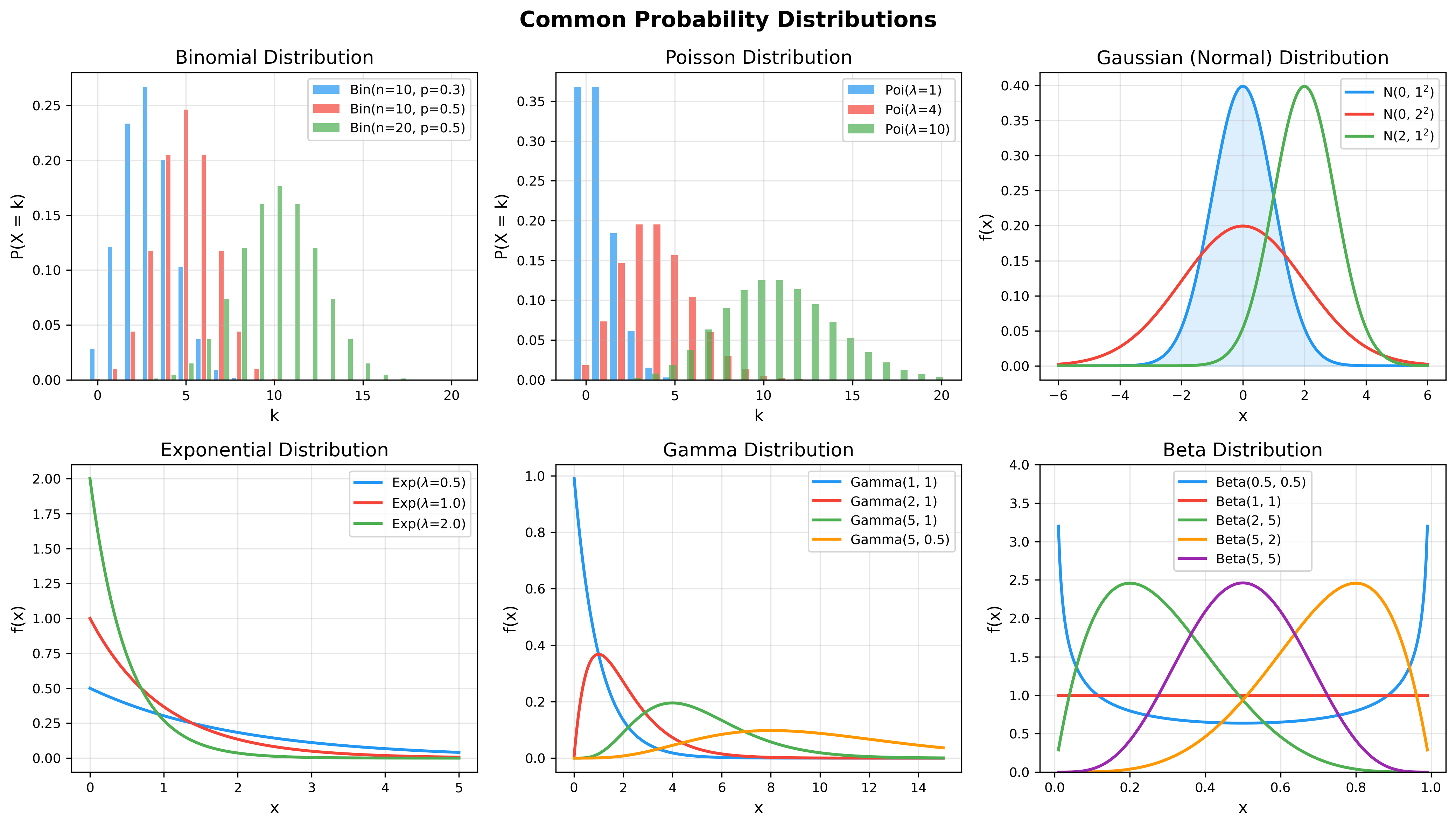
The following figure shows how distribution shapes change with different parameters — understanding parameter effects is key to choosing appropriate models:

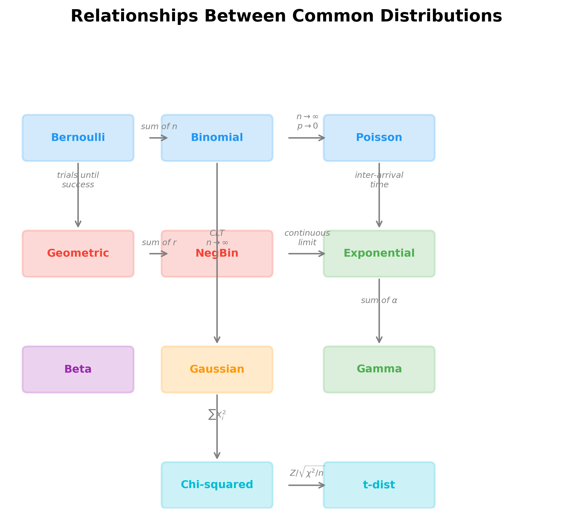
The diagram below illustrates the mathematical relationships between common distributions — these connections reveal deep structural ties in distribution theory:

Limit Theorems

Law of Large Numbers

Definition 18 (Convergence in Probability): Random variable sequenceconverges in probability to , denoted , if:

Theorem 15 (Markov's Inequality): If and , then for any :

Proof:

QED.

Theorem 16 (Chebyshev's Inequality): If , , then for any:

Proof: Apply Markov's inequality to:

QED.

Theorem 17 (Weak Law of Large Numbers, WLLN): Let be i.i.d. with , . Let, then:

Proof:

By Chebyshev's inequality:

QED.

Theorem 18 (Strong Law of Large Numbers, SLLN): Under WLLN conditions:

i.e., converges almost surely to, denoted.

Almost sure convergence vs convergence in probability:

Almost sure convergence (a.s.): sample path convergence
Convergence in probability: concentration of probability mass

Almost sure convergence is stronger than convergence in probability.

Central Limit Theorem

Theorem 19 (Central Limit Theorem, CLT): Let be i.i.d. with , . Let:

then:

wheredenotes convergence in distribution.

Proof sketch (using characteristic functions):

Let be standardized, so , .

Characteristic function of :

Taylor expansion of:

Therefore:

And is exactly the characteristic function of. By Lévy's continuity theorem, . QED.

Significance of CLT:

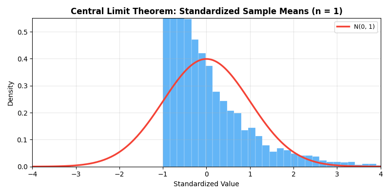
The animation below demonstrates the magic of the Central Limit Theorem — even when the original distribution is a highly skewed exponential distribution, as sample size increases, the standardized sample mean distribution gradually converges to the standard normal:

Explains why normal distribution is so prevalent: many phenomena are superposition of many small random effects
Provides theoretical foundation for statistical inference: distribution of sample mean approximately normal
Gives approximation error bound: Multivariate Central Limit Theorem: Letbe i.i.d. with,. Then:

Parameter Estimation

Point Estimation

Definition 19 (Estimator): Let be sample from distribution , where is unknown parameter. Estimatoris function of sample.

Definition 20 (Unbiasedness): If , then is unbiased estimator of.

Examples:

Sample mean is unbiased estimator of population mean
Sample variance is unbiased estimator of population variance

Why does sample variance divide by instead of ?

Proof of unbiasedness of sample variance:

Key step: .

Dividing bygives biased estimator:.

Definition 21 (Consistency): If, then is consistent estimator of.

Definition 22 (Mean Squared Error, MSE):

where.

Bias-variance decomposition:

Bias: systematic error of estimation
Variance: randomness of estimation
Tradeoff between them is core of statistical learning

Maximum Likelihood Estimation (MLE)

Definition 23 (Likelihood Function): Given sample , likelihood function is defined as:

Log-likelihood function:

Definition 24 (Maximum Likelihood Estimator): MLE is defined as:

Example 1: MLE for Bernoulli Distribution

Let . Likelihood function:

Log-likelihood:

Taking derivative:

Solving:

Example 2: MLE for Gaussian Distribution

Let . Log-likelihood:

Taking partial derivative with respect to:

Solving:

Note: This is biased! Unbiased estimator divides by .

Theorem 20 (Asymptotic Properties of MLE): Under regularity conditions, MLE has following properties:

Consistency:(true parameter)
Asymptotic normality:
Asymptotic efficiency: Among all consistent estimators, MLE achieves Cramér-Rao lower bound on asymptotic variance

where is Fisher information matrix:

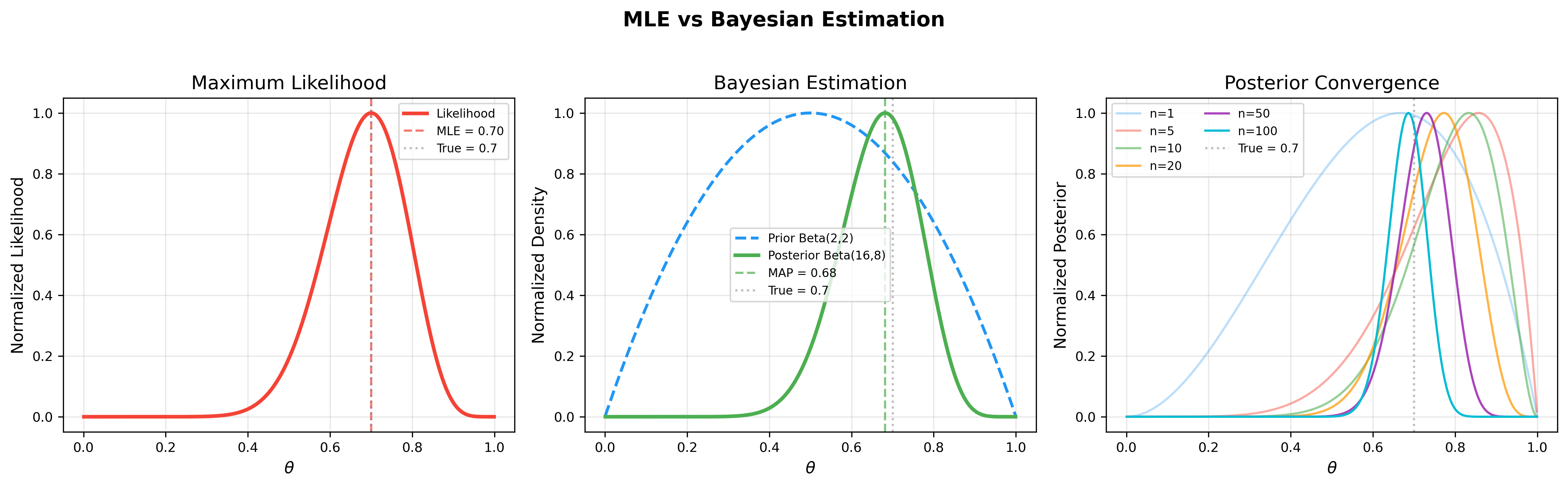
Bayesian Estimation

Bayesian paradigm: Treat parameteras random variable, assign prior distribution.

Posterior distribution: By Bayes' theorem:

Definition 25 (Posterior Mean Estimator):

Definition 26 (Maximum A Posteriori, MAP):

Example: Beta-Bernoulli Conjugacy

Prior:

Likelihood:

Posterior:

This is.

Posterior mean:

Interpretation:

Prior parameterscan be viewed as "pseudo-observations": prior believes there aresuccesses,failures
Posterior combines prior and data:successes,failures
As, posterior mean(MLE)

Bayesian vs Frequentist:

Feature	Frequentist	Bayesian
Parameter	Fixed but unknown	Random variable
Inference basis	Repeated sampling	Conditional probability
Prior knowledge	Not used	Explicitly modeled
Uncertainty	Confidence interval	Credible interval
Computation	Usually simpler	May need MCMC

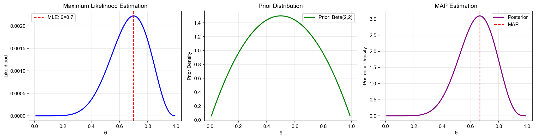
The figure below further illustrates the core Bayesian estimation workflow: the left panel shows the likelihood function, the middle panel shows how the prior distribution combines with the likelihood to produce the posterior, and the right panel demonstrates posterior convergence as data increases:

Hypothesis Testing and Confidence Intervals

Hypothesis Testing

Definition 27 (Statistical Hypothesis): Statement about population distribution.

Null hypothesis: default hypothesis (usually "no effect")
Alternative hypothesis: hypothesis researcher hopes to prove

Definition 28 (Test Statistic): Random variableconstructed from sample.

Definition 29 (Rejection Region): If, reject.

Two types of errors:

True State	Accept	Reject
true	✓	Type I error ()
true	Type II error ()	✓ (power)

Definition 30 (Significance Level):, typically 0.05 or 0.01.

Definition 31 (p-value): Under condition is true, probability of observing current or more extreme data:

Decision rule: If p-value, reject .

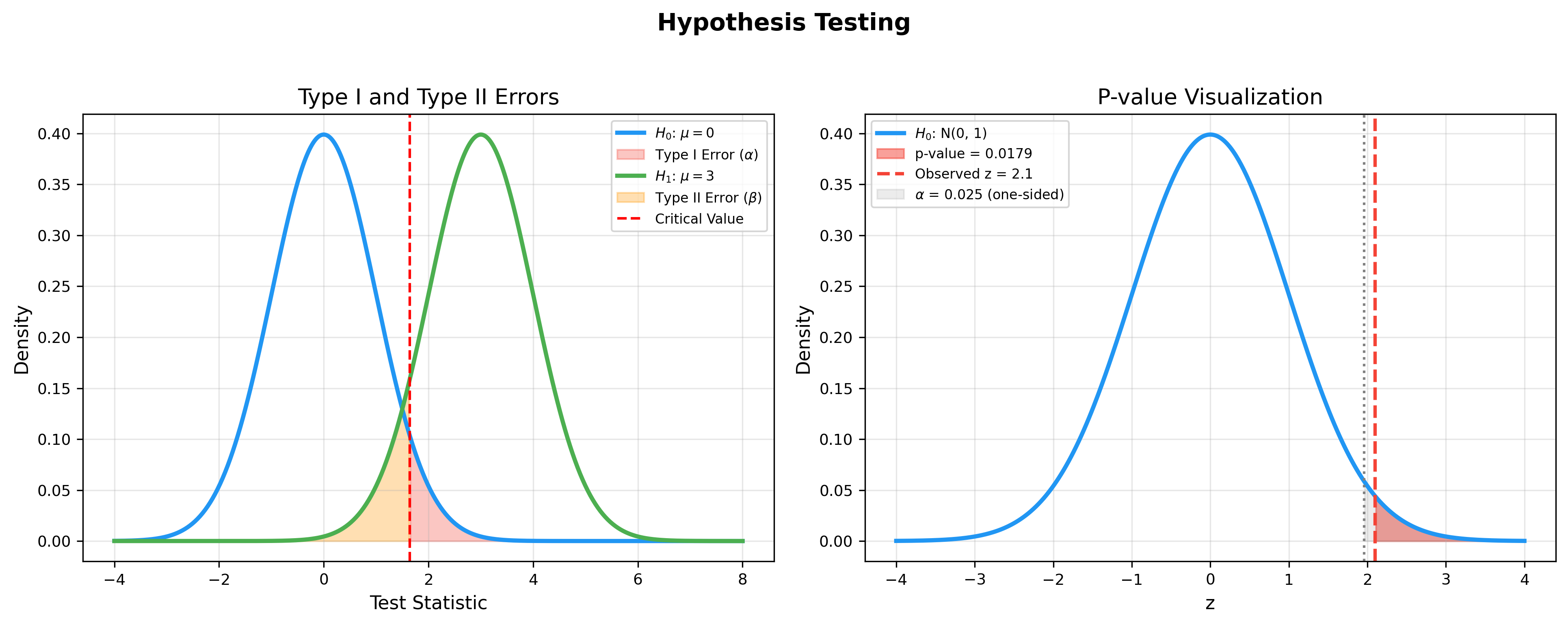
The figure below visualizes the core concepts of hypothesis testing: the left panel shows the trade-off between Type I error (rejecting a true ) and Type II error (failing to reject a false ); the right panel shows the geometric meaning of the p-value:

Example: One-sample t-test

Hypothesis: vs

Test statistic:

Under , .

Rejection region:, whereisquantile of t-distribution.

Confidence Intervals

Definition 32 (Confidence Interval): Random intervalis called confidence interval for if:

Note: This is probability statement about random interval, not about parameter (frequentist view).

Example: Confidence interval for mean

Let , known. By CLT:

Therefore:

Rearranging:

is confidence interval for.

Ifunknown, useinstead of, use t-distribution instead of normal: # ✏️ Exercises and Solutions

Exercise 1: Conditional Probability and Bayes' Formula

Problem: A disease has a prevalence of 0.1%. A test has sensitivity (true positive rate) of 99% and specificity (true negative rate) of 95%. If a person tests positive, what is the probability they actually have the disease?

Solution:

Let = disease, = positive test. Given: , , , so .

By Bayes' formula:

Even with a positive test, the actual probability of disease is only about 1.94%. This is a classic case of the "base rate fallacy" — when disease prevalence is very low, even an accurate test has low positive predictive value.

Exercise 2: Maximum Likelihood Estimation

Problem: Let be i.i.d. from uniform distribution , whereis unknown. Find the MLE of and determine whether it is unbiased.

Solution:

Likelihood function:

$𝟙 𝟙$

where .

To maximize , note is decreasing in, and we need. Therefore:

Checking unbiasedness: The CDF of is (), PDF is .

Therefore , so the MLE is biased (systematically underestimates).

Unbiased correction: .

Exercise 3: Central Limit Theorem Application

Problem: A machine produces screws with mean length 10mm and standard deviation 0.2mm. A random sample of 100 screws is taken. Find the probability that the sample mean falls in.

Solution:

Let be the length of the -th screw, , , .

By CLT, .

The probability of the sample mean falling inis approximately 95.44%.

Exercise 4: Bayesian Estimation with Conjugate Prior

Problem: A possibly unfair coin is flipped. Assume the prior for the probability of heads is. After 10 flips, 7 heads are observed. Find the posterior distribution and posterior mean of.

Solution:

Prior: .

Likelihood: , observed .

By Beta-Binomial conjugacy, the posterior is:

Posterior mean:

Compare with MLE: .

The posterior mean (0.643) is closer to 0.5 than the MLE (0.7), reflecting the "pull-back" effect of theprior (which favors a fair coin). As data size increases, the posterior mean converges to the MLE.

Exercise 5: Hypothesis Testing

Problem: A factory claims its products have mean weight 500g. A random sample of 25 products yields, . At significance level, test whether the claim holds.

Solution:

Set vs (two-sided test).

Test statistic:

Under , .

Critical value: .

Since, the test statistic does not fall in the rejection region. At significance level, we fail to reject .

p-value: .

Conclusion: There is insufficient statistical evidence to conclude the mean product weight differs significantly from 500g. Note: failing to reject does not prove is true — the sample size may be too small, resulting in insufficient statistical power.

Next chapter preview: Chapter 4 will delve into optimization theory foundations, including convex optimization, gradient descent, Newton's method, quasi-Newton methods, constrained optimization, etc., providing mathematical tools for training machine learning algorithms.