Machine Learning Mathematical Derivations (2): Linear Algebra and Matrix Theory

In Google's PageRank algorithm, the web ranking problem was transformed into a massive eigenvalue problem: finding the principal eigenvector of a transition matrix. Behind this elegant mathematical formulation lies the profound structure of linear algebra. Linear algebra is not merely the language of machine learning — it is the key to understanding the geometric structure of data.

Machine learning is fundamentally about finding optimal linear or nonlinear transformations in high-dimensional spaces. From the simplest linear regression (solving ), to complex deep neural networks (chains of matrix multiplications), to principal component analysis (eigenvalue decomposition), linear algebra is everywhere. This chapter derives all the linear algebra tools needed for machine learning from first principles.

Vector Spaces and Linear Transformations

Axiomatic Definition of Vector Spaces

Definition 1 (Vector Space): Letbe a non-empty set andbe a field (typicallyor). If two operations are defined on:

1. Vector addition:

2. Scalar multiplication:satisfying the following 8 axioms, thenis called a vector space over:

Addition axioms:

1. Commutativity:,

2. Associativity:,

3. Zero element:such that,

4. Inverse element: , such that

Scalar multiplication axioms:

5. Distributivity 1:,

6. Distributivity 2:,

7. Associativity:,

8. Identity: ,

Common vector space examples:

Space	Elements	Dimension	Application
	-dimensional real vectors		ML feature vectors
	-dimensional complex vectors		Quantum computing, signal processing
	real matrices		Data matrices, weight matrices
	Continuous functions on		Function approximation
	Polynomials of degree		Polynomial regression

Linear Independence and Basis

Definition 2 (Linear Combination): A vector can be expressed as a linear combination of vector setif there exist scalarssuch that:

Definition 3 (Linear Independence): A vector setis linearly independent if:

Otherwise, it is linearly dependent.

Theorem 1 (Equivalent Condition for Linear Dependence): A vector setis linearly dependent if and only if some vector can be expressed as a linear combination of others.

Proof: Suppose linearly dependent, then there exist not all zero such that. Without loss of generality, let, then:

Suppose , then, and coefficients are not all zero, hence linearly dependent. QED.

Definition 4 (Basis and Dimension): A basis of vector spaceis a linearly independent vector setsuch that any vector incan be uniquely expressed as a linear combination of these basis vectors. The number of basis vectors is called the dimension of the vector space, denoted.

Standard basis example:

Standard basis of:

Any can be uniquely expressed as .

Linear Transformations and Matrices

Definition 5 (Linear Transformation): Letbe two vector spaces. A mappingis called a linear transformation (or linear map) if:

1. Additivity:,

2. Homogeneity: ,

Theorem 2 (Matrix Representation of Linear Transformations): Let and be -dimensional and -dimensional vector spaces respectively, with chosen basesand. For a linear transformation , there exists a unique matrix such that for any :

where and are coordinate representations of vectors in their respective bases.

Proof:

Let , then:

by linearity. Now, can be expressed as a linear combination of 's basis:

Therefore:

This is exactly the -th component of matrix-vector multiplication , where . QED.

The -th column of matrix is exactly the coordinates of in 's basis. This is the geometric meaning of matrix representation.

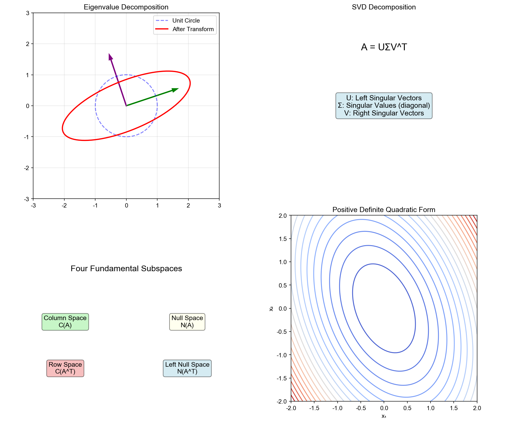
Four Fundamental Subspaces

For anmatrix, there are four fundamental subspaces that characterize its structure:

Definition 6 (Four Fundamental Subspaces):

1. Column Space:
   • Dimension:
   • Geometric meaning: All vectorscan reach
2. Null Space:
   • Dimension: (by rank-nullity theorem)
   • Geometric meaning: All vectors mapped to zero by
3. Row Space:
   • Dimension:
   • Geometric meaning: All vectorscan reach
4. Left Null Space:
   • Dimension:
   • Geometric meaning: Vectors orthogonal to row space

Theorem 3 (Orthogonality of Fundamental Subspaces):

1. (null space orthogonal to row space)
2. (left null space orthogonal to column space)

Proof of property 1:

Let , i.e., . For any , there exists such that . Compute inner product:

Therefore , i.e., . QED.

Dimension relations of fundamental subspaces:

These two equations show that and are each decomposed into two orthogonal subspaces.

Inner Product Spaces and Norms

Definition and Properties of Inner Products

Definition 7 (Inner Product): Letbe a real vector space. An inner product is a mappingsatisfying:

1. Symmetry:

2. Linearity:

3. Positive definiteness: , and

Common inner products:

1. Standard inner product (Euclidean inner product): For ,

2. Weighted inner product: Given positive definite diagonal matrix ,

3. Function space inner product: For ,

4. Matrix Frobenius inner product: For,

Definition and Properties of Norms

Definition 8 (Norm): A norm on vector spaceis a mappingsatisfying:

1. Positive definiteness:, and

2. Homogeneity:,

3. Triangle inequality: ,

Common vector norms:

1. norm: For , ,

Special cases: -norm (Manhattan distance): -norm (Euclidean norm): -norm (maximum norm):

2. Inner product induced norm: For inner product spaces,

Theorem 4 (Cauchy-Schwarz Inequality): For any in an inner product space,

Equality holds if and only if and are linearly dependent.

Proof:

For any , consider:

This is a quadratic function in , always non-negative. Therefore discriminant:

i.e., . Equality holds if and only if there exists such that , i.e., (linearly dependent). QED.

Corollaries of Cauchy-Schwarz inequality:

1. Triangle inequality:

Proof:

Taking square roots gives the triangle inequality.

2. Cosine formula:

where is the angle between and . By Cauchy-Schwarz inequality, .

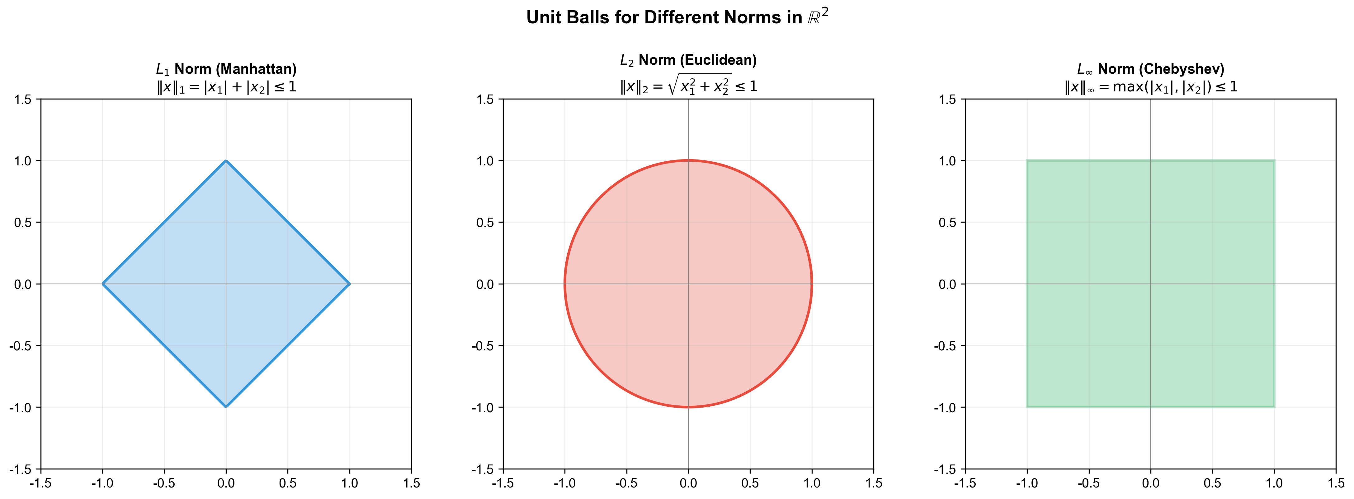
The figure below visualizes the unit balls of different norms in: the norm unit ball is a diamond, the norm unit ball is a circle, and the norm unit ball is a square. These geometric shapes directly determine the behavior of corresponding regularization methods (Lasso, Ridge):

Matrix Norms

Common Matrix Norms

Definition 9 (Matrix Norm): A matrix norm is a norm defined on matrix space.

Common matrix norms:

1. Frobenius norm:

2. Induced norm (operator norm): Induced by vector norms,

Special cases: - Spectral norm (2-norm): (largest singular value) - 1-norm: (maximum column sum) - -norm: (maximum row sum)

3. Nuclear norm (trace norm):

whereare singular values of .

Theorem 5 (Properties of Matrix Norms):

1. Submultiplicativity:(Frobenius norm doesn't satisfy this, but satisfies)

2. Submultiplicativity of induced norms:

3. Compatibility with vector norms: # Eigenvalues and Eigenvectors

Definition of Eigenvalue Problem

Definition 10 (Eigenvalues and Eigenvectors): Let . If there exists a non-zero vector and a scalarsuch that:

then is called an eigenvalue of , and is the corresponding eigenvector.

Computing eigenvalues:

Eigenvalues satisfy the characteristic equation:

This is an -th degree polynomial equation in, called the characteristic polynomial:

Theorem 6 (Properties of Eigenvalues):

1. (sum of eigenvalues equals trace)
2. (product of eigenvalues equals determinant)
3. is invertible all eigenvalues are non-zero
4. Eigenvalues of are
5. Similar matrices have same eigenvalues

Proof of properties 1 and 2:

The leading coefficient of characteristic polynomial is, the next coefficient is, and constant term is.

By Vieta's formulas, polynomialexpanded gives:

• Coefficient of:
• Constant term:

Comparing coefficients givesand. QED.

Spectral Theorem for Symmetric Matrices

Theorem 7 (Spectral Theorem for Symmetric Matrices): Let be a symmetric matrix, then:

1. All eigenvalues of are real
2. Eigenvectors corresponding to different eigenvalues are orthogonal
3. can be orthogonally diagonalized, i.e., there exist orthogonal matrix and diagonal matrix such that:

where, and columns of are orthonormal eigenvectors of .

Proof:

Step 1: Eigenvalues are real

Let , . Compute:

Therefore, i.e., .

Step 2: Eigenvectors for different eigenvalues are orthogonal

Let , , where. Compute:

Therefore. Since, we get .

Step 3: Orthogonal diagonalization

Since is an real symmetric matrix, it has eigenvalues (counting multiplicities) in the complex field. By Step 1, these eigenvalues are all real. For repeated eigenvalues, we can select an orthogonal basis in their eigenspace (Gram-Schmidt orthogonalization).

Therefore we can find orthonormal eigenvectors , forming orthogonal matrix . Then:

Multiplying both sides by on the right (using ), we get . QED.

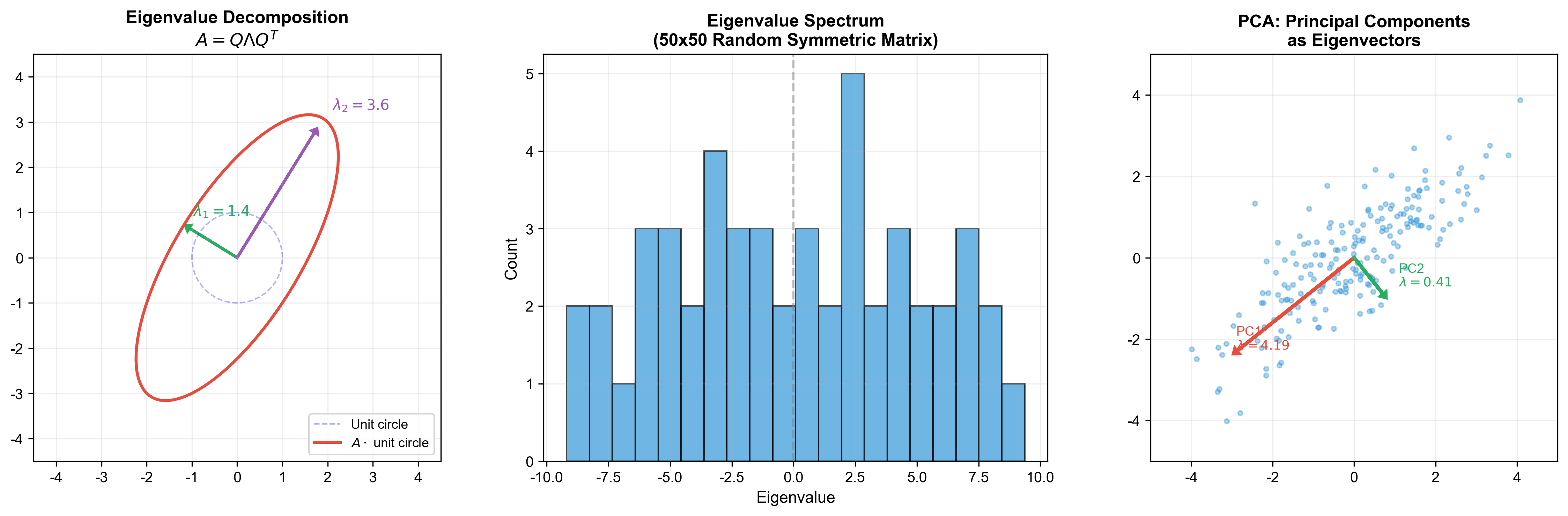
Geometric meaning of spectral decomposition:

This shows that can be decomposed as a weighted sum of rank-1 matrices, where each matrix is a projection along eigenvector , with weight being eigenvalue.

Positive Definite Matrices

Definition 11 (Positive Definite Matrix): A symmetric matrix is called positive definite if for all non-zero vectors ,

Similarly, we define positive semi-definite (), negative definite (), and negative semi-definite () matrices.

Theorem 8 (Equivalent Conditions for Positive Definiteness): The following are equivalent:

1. is positive definite
2. All eigenvalues of are positive
3. All leading principal minors of are positive
4. There exists an invertible matrix such that
5. Cholesky decomposition of exists: , where is lower triangular

Proof:

Let , . Then:

Therefore.

By spectral theorem, , where, . For any , let (since is invertible):

because at least one and all. QED.

Properties of positive definite matrices:

1. Positive definite matrices are always invertible
2. Inverse of positive definite matrix is also positive definite
3. Sum of two positive definite matrices is positive definite
4. Diagonal elements of positive definite matrix are all positive

The figure below illustrates the geometric meaning of eigenvalue decomposition: matrix transforms the unit circle into an ellipse, where the principal axes of the ellipse correspond to eigenvectors, and the axis lengths correspond to eigenvalues. The right panel shows that eigenvectors point in the principal directions of data (the core idea behind PCA):

Eigenvalue Visualization

Singular Value Decomposition (SVD)

SVD Theorem and Geometric Meaning

Theorem 9 (Singular Value Decomposition): Let with rank . Then there exist orthogonal matrices and , and diagonal matrix, such that:

where diagonal elementsof are called singular values of .

Full form:

Compact form (economy SVD):

where , , .

Proof sketch:

Step 1: Inspiration from eigenvalue decomposition

Considerand:

• is symmetric positive semi-definite
• is symmetric positive semi-definite

By spectral theorem, they can be orthogonally diagonalized.

Step 2: Right singular vectors (from )

Eigenvalue decomposition of :

where columns of , , are orthonormal eigenvectors of , , .

Defineas singular values (ordered decreasingly).

Step 3: Construction of left singular vectors

For (where), define:

Verify orthogonality of :

For , extendto an orthonormal basis of using Gram-Schmidt orthogonalization.

Step 4: Verify

For :

For :

(because , i.e., implies)

Therefore:

Multiplying both sides by on the right gives . QED.

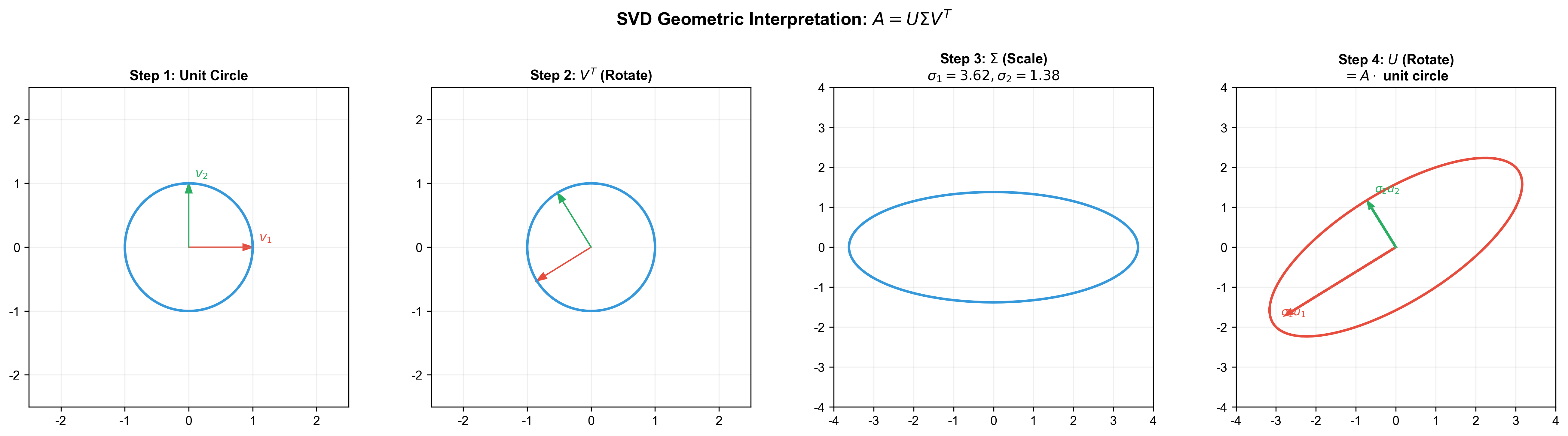
Geometric meaning of SVD:

Any linear transformation can be decomposed into three steps:

1. Rotation (or reflection): rotates's standard orthonormal basis to eigenvector basis of

2. Scaling: scales along directions, with scaling factors being singular values

3. Rotation (or reflection): rotates result to's standard orthonormal basis

Linear Algebra Core Concepts

Applications of SVD

1. Low-Rank Approximation

Theorem 10 (Eckart-Young Theorem): Let be SVD of , and be rank approximation. Then is the best approximation to among all rank matrices in both Frobenius norm and spectral norm:

Proof sketch (spectral norm):

Let be any rank matrix. Then. Considerand:

But they are both subspaces of, so there must exist a non-zero intersection. There exists , .

Since , , . Then:

More refined arguments (using minimax principle) prove, and achieves this lower bound.

Application: Principal Component Analysis (PCA)

Given centered data matrix (each column has mean 0), perform SVD on :

Take first principal components:

This is the best rank approximation of , i.e., reducing data from dimensions to dimensions while preserving maximum variance.

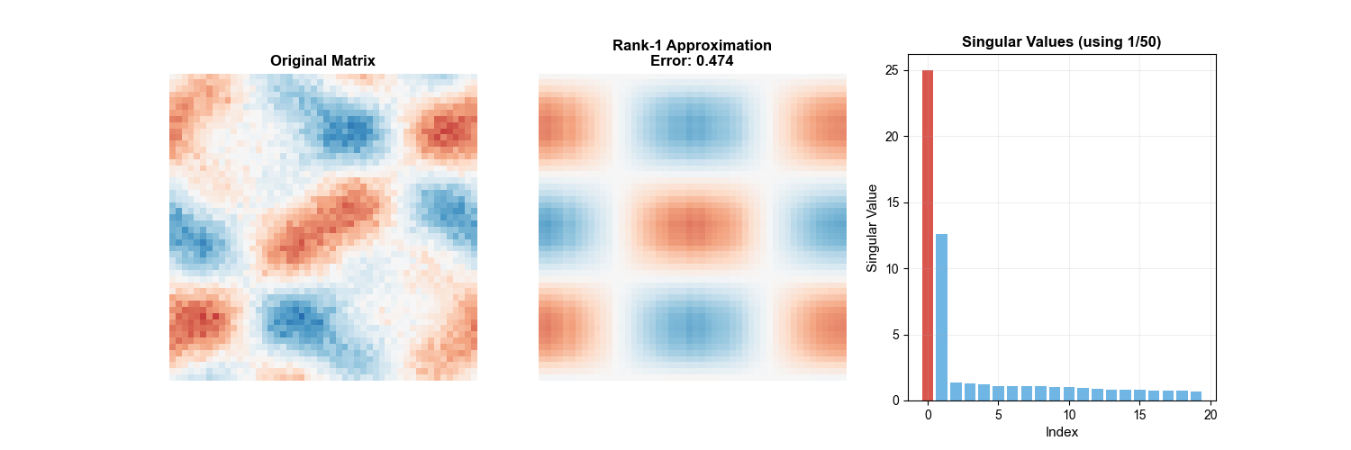
The figure below visualizes the geometric meaning of SVD decomposition: any matrix transforms the unit circle into an ellipse through rotation and scaling, where singular values determine the length of each axis:

SVD Visualization

The following animation intuitively demonstrates the SVD low-rank approximation process — as the number of retained singular values increases, the approximation quality improves continuously, which is a practical manifestation of the Eckart-Young theorem:

SVD Truncation Animation

2. Pseudoinverse Matrix

Definition 12 (Moore-Penrose Pseudoinverse): The pseudoinverse of matrix is the unique matrix satisfying these four properties:

Theorem 11 (Computing Pseudoinverse via SVD): Let be SVD of , then:

whereis defined as:

i.e., .

Verification:

Verify that satisfies the four properties. Taking property 1 as example:

because (first diagonal elements are 1). Other properties verified similarly.

Least squares solution:

For inconsistent system , the least squares solution is:

This is the minimum norm least squares solution among all solutions minimizing.

3. Condition Number

Definition 13 (Condition Number): The condition number of matrix is defined as:

Condition number measures the "ill-conditioning" of a matrix. Largermeans system is more sensitive to perturbations in .

Theorem 12 (Perturbation Bound): Let , , then:

This shows relative error is amplified by condition number.

Matrix Calculus

Matrix calculus is ubiquitous in machine learning optimization. This section derives common matrix calculus formulas from first principles.

Notation for Matrix Calculus

Scalar with respect to vector:

Let , then derivative of with respect to vector is defined as:

This is called the gradient vector, denoted or.

Scalar with respect to matrix:

Let , then derivative of with respect to matrix is defined as:

Vector with respect to vector:

Let,, then the Jacobian matrix is defined as:

Note: Matrix calculus notation conventions may differ across literatures (numerator layout vs denominator layout). This chapter uses numerator layout, where derivative shape matches numerator (function being differentiated) shape.

Basic Derivative Formulas

1. Linear Functions

Formula 1: , then:

Proof:

Therefore:

i.e., .

2. Quadratic Form

Formula 2: (where ), then:

In particular, if is symmetric:

Proof:

Differentiating with respect to :

Therefore. When , we get. QED.

3. Matrix Multiplication

Formula 3: (where , , ), then:

Proof:

Differentiating with respect to :

Therefore. QED.

4. Trace of Matrix

Formula 4: (where , ), then:

In particular, if is symmetric:

Proof:

Using cyclic property of trace:

Direct computation:

Therefore. QED.

5. Determinant and Inverse

Formula 5: (where is invertible), then:

Proof:

Using chain rule and:

For determinant differential, there is formula (Jacobi's formula):

Therefore:

By relation between differential and derivative , we get:

QED.

Formula 6: , then:

where is matrix with 1 atposition and 0 elsewhere.

Chain Rule and Backpropagation

Theorem 13 (Chain Rule for Scalar Functions): Let , , then composite function has derivative:

whereis Jacobian matrix.

Proof:

By multivariate chain rule:

In matrix form:

QED.

Backpropagation example:

Consider one layer of neural network:

where , , , is activation function (element-wise).

Let loss function be . To compute:

Let , then:

But this involves matrix-to-matrix differentiation, requiring more careful treatment. Actually:

Note that , so (Kronecker delta).

Therefore:

whereis "error signal" of -th neuron.

In matrix form:

where.

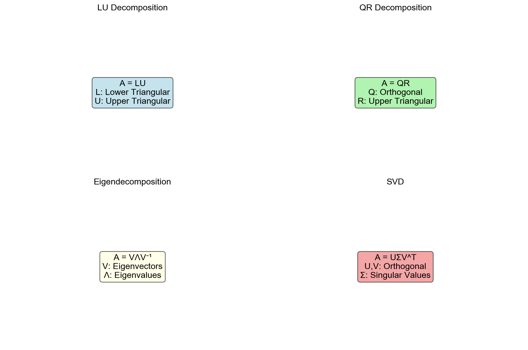
Numerical Computation of Matrix Decompositions

QR Decomposition

Theorem 14 (QR Decomposition): Let () be full column rank, then there exist orthogonal matrix and upper triangular matrix such that:

Gram-Schmidt orthogonalization algorithm:

Given linearly independent vectors, construct orthonormal vectors:

Then:

In matrix form:

where , ().

Applications of QR decomposition:

1. Solving least squares: Solution is (using ).

2. Computing eigenvalues: QR iteration algorithm

   Repeat:

Under certain conditions, converges to upper triangular matrix, with eigenvalues on diagonal.

Cholesky Decomposition

Theorem 15 (Cholesky Decomposition): Let be positive definite, then there exists unique lower triangular matrix (with positive diagonal) such that:

Algorithm:

Recursively compute elements of :

Computational complexity: (twice as fast as LU decomposition)

Applications:

1. Solving linear system :
   • Decompose
   • Solve (forward substitution)
   • Solve (backward substitution)
2. Testing positive definiteness: If Cholesky decomposition succeeds (all positive), then is positive definite.

Code Implementation: Matrix Decompositions and Applications

import numpy as np
import matplotlib.pyplot as plt
from scipy.linalg import svd, qr, cholesky
import time

# Set random seed
np.random.seed(42)

def demonstrate_svd():
    """
    Demonstrate SVD decomposition and low-rank approximation
    """
    print("="*60)
    print("1. Singular Value Decomposition (SVD) and Low-Rank Approximation")
    print("="*60)
    
    # Create low-rank matrix + noise
    m, n = 100, 80
    rank_true = 10
    
    # True low-rank matrix: A = U @ S @ V^T
    U_true = np.random.randn(m, rank_true)
    S_true = np.diag(np.linspace(10, 1, rank_true))  # Decreasing singular values
    V_true = np.random.randn(n, rank_true)
    A_true = U_true @ S_true @ V_true.T
    
    # Add noise
    noise_level = 0.5
    A_noisy = A_true + noise_level * np.random.randn(m, n)
    
    # SVD decomposition
    U, s, Vt = svd(A_noisy, full_matrices=False)
    
    print(f"Original matrix shape: {A_noisy.shape}")
    print(f"First 10 singular values: {s[:10]}")
    print(f"Last 10 singular values: {s[-10:]}")
    
    # Low-rank approximation
    ranks = [1, 5, 10, 20, 40]
    errors_fro = []
    errors_spec = []
    
    for k in ranks:
        # Rank-k approximation: A_k = U[:, :k] @ diag(s[:k]) @ Vt[:k, :]
        A_k = U[:, :k] @ np.diag(s[:k]) @ Vt[:k, :]
        
        error_fro = np.linalg.norm(A_noisy - A_k, 'fro')
        error_spec = np.linalg.norm(A_noisy - A_k, 2)
        
        errors_fro.append(error_fro)
        errors_spec.append(error_spec)
        
        print(f"Rank-{k} approximation: Frobenius error={error_fro:.2f}, Spectral error={error_spec:.2f}")
    
    # Theoretical predictions
    print("\nTheoretical predictions (Eckart-Young theorem):")
    for i, k in enumerate(ranks):
        theory_fro = np.sqrt(np.sum(s[k:]**2))
        theory_spec = s[k] if k < len(s) else 0
        print(f"Rank-{k}: Theory Fro error={theory_fro:.2f}, Theory spectral error={theory_spec:.2f}")
    
    # Plotting
    plt.figure(figsize=(12, 4))
    
    plt.subplot(1, 2, 1)
    plt.semilogy(np.arange(1, len(s)+1), s, 'o-')
    plt.xlabel('Singular Value Index')
    plt.ylabel('Singular Value (log scale)')
    plt.title('SVD Singular Value Spectrum')
    plt.grid(True, alpha=0.3)
    
    plt.subplot(1, 2, 2)
    plt.plot(ranks, errors_fro, 'o-', label='Frobenius Error')
    plt.plot(ranks, errors_spec, 's-', label='Spectral Error')
    plt.xlabel('Approximation Rank')
    plt.ylabel('Approximation Error')
    plt.title('Low-Rank Approximation Error')
    plt.legend()
    plt.grid(True, alpha=0.3)
    
    plt.tight_layout()
    plt.savefig('svd_demo.png', dpi=150)
    plt.close()
    
    print("\nFigure saved as svd_demo.png\n")

def demonstrate_qr():
    """
    Demonstrate QR decomposition and its application to least squares
    """
    print("="*60)
    print("2. QR Decomposition and Least Squares Problems")
    print("="*60)
    
    # Generate overdetermined system Ax = b (m > n)
    m, n = 100, 10
    A = np.random.randn(m, n)
    x_true = np.random.randn(n)
    b = A @ x_true + 0.1 * np.random.randn(m)  # Add noise
    
    # Method 1: Normal equations x = (A^T A)^(-1) A^T b
    start = time.time()
    x_normal = np.linalg.solve(A.T @ A, A.T @ b)
    time_normal = time.time() - start
    
    # Method 2: QR decomposition A = QR, solve Rx = Q^T b
    start = time.time()
    Q, R = qr(A, mode='economic')
    x_qr = np.linalg.solve(R, Q.T @ b)
    time_qr = time.time() - start
    
    # Method 3: SVD pseudoinverse x = A^+ b
    start = time.time()
    x_svd = np.linalg.lstsq(A, b, rcond=None)[0]
    time_svd = time.time() - start
    
    print(f"True solution x_true: {x_true[:5]}...")
    print(f"Normal equations: {x_normal[:5]}... (time {time_normal*1000:.2f}ms)")
    print(f"QR decomposition: {x_qr[:5]}... (time {time_qr*1000:.2f}ms)")
    print(f"SVD pseudoinverse: {x_svd[:5]}... (time {time_svd*1000:.2f}ms)")
    
    # Residual comparison
    print(f"\nResidual norms:")
    print(f"Normal equations: {np.linalg.norm(A @ x_normal - b):.6f}")
    print(f"QR decomposition: {np.linalg.norm(A @ x_qr - b):.6f}")
    print(f"SVD pseudoinverse: {np.linalg.norm(A @ x_svd - b):.6f}")
    
    # Condition number analysis
    kappa = np.linalg.cond(A)
    kappa_ata = np.linalg.cond(A.T @ A)
    print(f"\nCondition number κ(A) = {kappa:.2f}")
    print(f"Condition number κ(A^T A) = {kappa_ata:.2f} ≈ κ(A)^2")
    print("Conclusion: QR decomposition has better numerical stability (no A^T A)\n")

def demonstrate_cholesky():
    """
    Demonstrate Cholesky decomposition
    """
    print("="*60)
    print("3. Cholesky Decomposition (Positive Definite Matrices)")
    print("="*60)
    
    # Generate positive definite matrix A = B^T B
    n = 50
    B = np.random.randn(n, n)
    A = B.T @ B + np.eye(n)  # Add identity to ensure positive definiteness
    
    # Cholesky decomposition A = L L^T
    start = time.time()
    L = cholesky(A, lower=True)
    time_chol = time.time() - start
    
    # Verification
    error = np.linalg.norm(A - L @ L.T, 'fro')
    print(f"Cholesky decomposition time: {time_chol*1000:.2f}ms")
    print(f"Reconstruction error ||A - LL^T||_F = {error:.2e}")
    
    # Application: Solving linear system Ax = b
    b = np.random.randn(n)
    
    # Method 1: Direct solve
    start = time.time()
    x_inv = np.linalg.solve(A, b)
    time_inv = time.time() - start
    
    # Method 2: Cholesky decomposition + forward/backward substitution
    start = time.time()
    y = np.linalg.solve(L, b)  # Forward substitution Ly = b
    x_chol = np.linalg.solve(L.T, y)  # Backward substitution L^T x = y
    time_chol_solve = time.time() - start
    
    print(f"\nSolving Ax = b:")
    print(f"Direct solve time: {time_inv*1000:.2f}ms")
    print(f"Cholesky solve time: {time_chol_solve*1000:.2f}ms")
    print(f"Solution error: {np.linalg.norm(x_inv - x_chol):.2e}")
    print("Conclusion: Cholesky decomposition is faster (complexity O(n^3/3) vs O(n^3))\n")

def demonstrate_matrix_calculus():
    """
    Demonstrate matrix calculus in ML: gradient computation for linear regression
    """
    print("="*60)
    print("4. Matrix Calculus: Gradient Computation for Linear Regression")
    print("="*60)
    
    # Generate linear regression data
    n, d = 100, 5
    X = np.random.randn(n, d)
    w_true = np.random.randn(d)
    y = X @ w_true + 0.1 * np.random.randn(n)
    
    # Loss function: L(w) = (1/2n) ||Xw - y||^2
    def loss(w):
        return 0.5 / n * np.sum((X @ w - y)**2)
    
    # Analytic gradient: ∂ L/∂ w = (1/n) X^T (Xw - y)
    def gradient_analytic(w):
        return 1/n * X.T @ (X @ w - y)
    
    # Numerical gradient (for verification)
    def gradient_numeric(w, eps=1e-7):
        grad = np.zeros_like(w)
        for i in range(len(w)):
            w_plus = w.copy()
            w_plus[i] += eps
            w_minus = w.copy()
            w_minus[i] -= eps
            grad[i] = (loss(w_plus) - loss(w_minus)) / (2 * eps)
        return grad
    
    # Test point
    w_test = np.random.randn(d)
    
    grad_ana = gradient_analytic(w_test)
    grad_num = gradient_numeric(w_test)
    
    print(f"Analytic gradient: {grad_ana}")
    print(f"Numeric gradient: {grad_num}")
    print(f"Error: {np.linalg.norm(grad_ana - grad_num):.2e}")
    print("Conclusion: Analytic gradient matches numerical gradient\n")
    
    # Gradient descent
    w = np.zeros(d)
    lr = 0.1
    losses = []
    
    for epoch in range(100):
        grad = gradient_analytic(w)
        w = w - lr * grad
        losses.append(loss(w))
    
    print(f"True weights: {w_true}")
    print(f"Learned weights: {w}")
    print(f"Initial loss: {losses[0]:.4f}")
    print(f"Final loss: {losses[-1]:.4f}")
    
    # Analytic solution: w* = (X^T X)^(-1) X^T y
    w_analytic = np.linalg.solve(X.T @ X, X.T @ y)
    print(f"Analytic solution: {w_analytic}")
    print(f"Gradient descent vs analytic error: {np.linalg.norm(w - w_analytic):.2e}\n")

if __name__ == "__main__":
    print("╔" + "="*58 + "╗")
    print("║" + " "*10 + "Linear Algebra and Matrix Theory Experiments" + " "*2 + "║")
    print("╚" + "="*58 + "╝")
    print()
    
    demonstrate_svd()
    demonstrate_qr()
    demonstrate_cholesky()
    demonstrate_matrix_calculus()
    
    print("="*60)
    print("All experiments completed!")
    print("="*60)

Code walkthrough:

1. SVD demonstration:
   • Verifies Eckart-Young theorem: rank-approximation error equals sum of squares from-th singular value onwards
   • Shows singular value spectrum: true signal's singular values decay rapidly, noise singular values are flat
2. QR decomposition demonstration:
   • Compares three methods for solving least squares: normal equations, QR decomposition, SVD pseudoinverse
   • Shows numerical stability advantage of QR decomposition (no need to compute, condition number doesn't square)
3. Cholesky decomposition demonstration:
   • Verifies accuracy of
   • Shows speed advantage of Cholesky decomposition for solving positive definite linear systems
4. Matrix calculus demonstration:
   • Verifies analytic gradient formula for linear regression matches numerical gradient
   • Implements gradient descent and compares with analytic solution

❓ Q&A: Common Questions on Linear Algebra

Q1: Why does SVD always exist while eigenvalue decomposition may not?

Key difference:

Property	Eigenvalue Decomposition	Singular Value Decomposition
Applicable matrices	Square	Any
Decomposition form
Left/right vectors	Same ()	Different (,)
Existence	Only for diagonalizable matrices	Always exists
Value properties	Eigenvalues may be complex	Singular values always non-negative real

Why does SVD always exist?

SVD construction doesn't depend on's structure, but onand:

-is symmetric positive semi-definite -is symmetric positive semi-definite

Spectral theorem for symmetric matrices guarantees they can be orthogonally diagonalized, so SVD always exists.

When doesn't eigenvalue decomposition exist?

Non-symmetric square matrices may not be diagonalizable. For example:

Eigenvalues: (repeated eigenvalue)

Eigenvectors: Only one linearly independent eigenvector, cannot form basis for.

Thereforeis not diagonalizable, eigenvalue decomposition doesn't exist (only Jordan normal form exists).

Practical applications:

• SVD applies to any data matrix, widely used in PCA, recommender systems, image compression
• Eigenvalue decomposition used for symmetric matrices (covariance matrices, graph Laplacians) or iterative solving problems

Matrix Decomposition Comparison

---

Q2: When should QR decomposition be used instead of normal equations for least squares?

Numerical stability issue of normal equations:

Normal equationsrequire computing, which causes condition number to square:

Numerical example:

Supposehas condition number(moderately ill-conditioned). Then:

-'s relative error may be amplifiedtimes -'s relative error may be amplifiedtimes

In finite precision arithmetic (e.g., double precision floating point, relative precision):

• Using normal equations: lose about 6 significant digits, result may have only 10 significant digits
• Using QR decomposition: lose about 3 significant digits, result has 13 significant digits

Practical example:

Consider matrix:

In double precision, term gets rounded off, making nearly singular, unable to solve accurately.

But QR decomposition works directly on, doesn't involve, numerically stable.

Recommendations:

• ✅ For ill-conditioned problems with, use QR decomposition or SVD
• ✅ For tall-thin matrices with, QR decomposition is more efficient
• ⚠️ Only use normal equations whenhas small condition number () andnot too large

---

Q3: How to understand matrix rank? Why is rank important?

Multiple equivalent definitions of rank:

1. Column space dimension:

2. Row space dimension:

3. Number of linearly independent columns: Size of maximal linearly independent column set

4. Number of non-zero singular values:

Geometric meaning:

Rank is the "effective dimension" of matrixas a linear transformation:

-meansmaps-dimensional space to an-dimensional subspace of-dimensional space - Dimension "loss" =(null space dimension)

Why is rank important?

1. Invertibility: -is invertible

2. Equation solvability: -has solution

   • Solution unique

3. Degrees of freedom:

   • General solution of homogeneous equationhasfree parameters

4. Data dimensionality reduction:

   • PCA projects data onto rank-subspace, preserving maximum variance

Practical applications:

Domain	Meaning of Rank
Machine Learning	Effective dimension of features
Recommender Systems	Number of latent factors in user-item interaction matrix
Image Compression	Low-rank approximation of image matrix
Control Theory	Controllability/observability of system

Numerical rank:

Due to floating point errors, numerical rank is defined as:

where is threshold (e.g., ).

---

Q4: What's the relationship between inner products and norms? Why do we need different norms?

Inner product induced norm:

For inner product spaces, inner product naturally induces a norm:

For example, standard inner product induces norm.

Not all norms come from inner products:normandnormcannot be induced by any inner product.

Testing if norm comes from inner product: Parallelogram law

Normis induced by inner productsatisfies parallelogram law: norm satisfies this law,anddon't.

Applications of different norms:

Norm	Geometric Meaning	Application
	Manhattan distance, diamond contours	Sparse regularization (Lasso)
	Euclidean distance, circular contours	Ridge regression, SVM
	Chebyshev distance, square contours	Robust optimization, minimax
	Number of non-zero elements (not a norm)	Feature selection, compressed sensing

Why doesproduce sparse solutions?norm's level sets have corners at coordinate axes. When constraint set (e.g.,) intersects objective function's level sets, intersection point tends to be on coordinate axes (some components zero), producing sparse solutions.

Illustration:

L1 constraint (diamond)    L2 constraint (circle)
      w2                       w2
       |                        |
      /|\                      / \
     / | \                    /   \
    /  |  \                  |     |
   ----+----w1              -------w1
    \  |  /                  |     |
     \ | /                    \   /
      \|/                      \ /

L1 constraint's corners more easily touch coordinate axes (sparse solutions).

---

Q5: Why are positive definite matrices so important in machine learning?

Core properties of positive definite matrices:

Symmetric positive definite matrixsatisfies:

1. All eigenvalues
2. For all ,
3. Can be written as (e.g., Cholesky decomposition )

Role in optimization:

Theorem: Functionis convexis positive semi-definite

Proof: Hessian matrix. Function convexHessian positive semi-definite.

Strictly convex function (unique optimal solution):positive definitestrictly convexunique global minimum.

Practical applications:

1. Normal equations in linear regression:

is positive semi-definite. Ifis full column rank,is positive definite, equation has unique solution.

2. Kernel matrices: Gram matrixcorresponding to kernel functionmust be positive definite (Mercer's theorem).

3. Covariance matrices: Data covariance matrixis always positive semi-definite.

4. Second-order optimization: Newton's method, conjugate gradient method depend on Hessian positive definiteness.

Meaning of negative definite matrices:

Function(positive definite) is concave, used for maximization problems.

Testing positive definiteness:

1. Eigenvalues: All eigenvalues

2. Sylvester's criterion: All leading principal minors

3. Cholesky decomposition: Try decomposition, success means positive definite

4. Numerical method: Compute minimum eigenvalue

---

Q6: What's the difference between "numerator layout" and "denominator layout" in matrix calculus?

Two layout conventions:

Layout	Rule	shape	Common in
Numerator	Derivative shape matches numerator	Same asshape	Statistics, ML
Denominator	Derivative shape matches denominator	Same asshape (transposed)	Physics, engineering

Example:

Let,, Jacobian matrix:

• Numerator layout:
• Denominator layout:

Scalar with respect to vector:

Let.

• Numerator layout:(column vector)
• Denominator layout:(row vector)

Comparison of important formulas:

Formula	Numerator Layout	Denominator Layout

Convention in this chapter:

This chapter uses numerator layout, because:

1. Consistent with natural vector/matrix shape
2. More common in ML literature
3. Gradient is column vector, convenient for gradient descent

Practical recommendations:

• ✅ When reading papers, first determine author's layout convention
• ✅ Stay consistent in your own code/derivations
• ✅ Use automatic differentiation libraries (PyTorch, JAX) to avoid manual derivation

---

Q7: How to quickly determine if a matrix is invertible?

Theoretical criteria:

Matrixis invertibleany of these conditions holds:

1. 2. 3. (null space contains only zero vector) 4. All eigenvalues non-zero 5. Row vectors (or column vectors) linearly independent 6.can be reduced to identity matrix through row operations

Numerical criteria (practical computation):

Due to floating point errors, use:

1. Condition number:
   • : numerically invertible
   • : numerically singular
2. Minimum singular value:
   • (where): invertible
3. LU decomposition: Try LU decomposition, if encounter zero pivot (or extremely small pivot), matrix singular

Quick checks (without full computation):

def is_invertible_quick(A, tol=1e-10):
    """
    Quickly determine if matrix is numerically invertible
    """
    # Method 1: Check determinant (only for small matrices)
    if A.shape[0] <= 10:
        return abs(np.linalg.det(A)) > tol
    
    # Method 2: Check condition number
    kappa = np.linalg.cond(A)
    return kappa < 1 / tol
    
    # Method 3: Try solving Ax=b
    try:
        x = np.linalg.solve(A, np.ones(A.shape[0]))
        residual = np.linalg.norm(A @ x - np.ones(A.shape[0]))
        return residual < tol
    except np.linalg.LinAlgError:
        return False

Invertibility of special matrices:

Matrix Type	Invertibility Condition
Diagonal	All diagonal elements non-zero
Triangular	All diagonal elements non-zero
Orthogonal	Always invertible ()
Symmetric positive definite	Always invertible
Idempotent ()	Only when

---

Q8: What's the relationship between SVD and PCA? Why does PCA use eigenvalue decomposition of covariance matrix?

Two equivalent derivations of PCA:

Method 1: Maximum variance (eigenvalue decomposition of covariance matrix)

Given centered data matrix(each column has mean 0).

Objective: Find direction,, maximizing data variance along this direction.

Variance:whereis covariance matrix.

Optimization problem:

By Lagrange multipliers, optimal solution satisfies:

i.e., is eigenvector of, is eigenvalue. Maximum variance corresponds to largest eigenvalue.

Method 2: Minimum reconstruction error (SVD of data matrix)

Objective: Find rank-matrixminimizing.

By Eckart-Young theorem, optimal solution is rank-SVD approximation of:

whereare firstright singular vectors, exactly the firsteigenvectors of(covariance matrix times).

Equivalence of two methods:

i.e.:

• Right singular vectors of= eigenvectors of(PCA principal directions)
• Squared singular values of= eigenvalues of(explained variance)

Choice in practical computation:

Method	Formula	Applicable Scenario
Eigenvalue decomposition of covariance matrix		(many samples, few features)
SVD of data matrix		(high-dimensional data, e.g., images)

Why is SVD better for high dimensions?

• Covariance matrix:, requirestime
• Data matrix SVD:, economy SVD only requirestime

When(e.g., image pixels, samples), SVD is much faster.

---

Q9: Why are rank-1 matrices called "atoms of matrices"?

Definition of rank-1 matrix:

Matrixis rank-1 if.

Equivalent condition:can be written as outer product of two vectors:

Why called "atoms"?

Any matrix can be decomposed as sum of rank-1 matrices. This is analogous to:

• Vectors can be decomposed as linear combinations of basis vectors
• Functions can be decomposed as Fourier series (sum of sine/cosine functions)

SVD rank-1 decomposition:

Each term is rank-1 matrix, is weighted sum of rank-1 matrices.

Properties of rank-1 matrices:

1. Simple structure:completely determined by two vectors
2. Low storage: Storingmatrix requiresnumbers, rank-1 matrix only needsnumbers
3. Fast multiplication:, first compute inner product(O(n)), then scale (O(m)), total O(m+n), much less than O(mn)

Applications:

1. Low-rank matrix completion (recommender systems): User-item rating matrix approximated as rank- matrix (k small):

2. Neural network compression: Weight matrixapproximated by rank-, parameters reduced fromto.

3. Fast matrix multiplication: If, then, computation fromto.

---

Q10: What's the relationship between Gram matrix () and Gram-Schmidt orthogonalization?

Definition of Gram matrix:

Given matrix , Gram matrix is defined as:

Elements:

i.e., inner products between column vectors.

Properties of Gram matrix:

1. Symmetric:

2. Positive semi-definite:

3. Rank:

4. Invertibility:invertiblefull column rank

Gram-Schmidt orthogonalization:

Objective: Transforminto orthonormal basis.

Process:

Relationship:

Gram-Schmidt orthogonalization essentially "removes projection ofonto subspace spanned by firstvectors", equivalent to:

1. Compute projection:
2. Compute orthogonal component:
3. Normalize

Cholesky decomposition of Gram matrix:

Ifis full column rank, thenis positive definite, can be Cholesky decomposed:

whereis lower triangular. Actually, columns ofare proportional to intermediate vectors in Gram-Schmidt process (unnormalized).

Numerical stability:

Classical Gram-Schmidt (CGS) is numerically unstable: subsequent vectors may not be orthogonal.

Modified Gram-Schmidt (MGS) is more stable: orthogonalize one vector at a time.

Relationship between QR decomposition and Gram-Schmidt:

QR decompositioncan be obtained through Gram-Schmidt:

• Columns of are orthogonalized vectors
• is upper triangular, elements are

Conversely, Gram matrix can be expressed through QR:

This is exactly Cholesky decomposition of Gram matrix!

🎓 Summary: Core Points of Linear Algebra

Key formulas to remember:

1. Four fundamental subspaces:

2. SVD decomposition:

3. Spectral theorem (symmetric matrices):

4. Matrix calculus:

Memory mnemonic:

SVD is universal key (any matrix decomposable)

Symmetric matrices have real eigenvalues (spectral theorem guarantees orthogonality)

Positive definite matrices optimize well (convex functions have unique solutions)

QR decomposition is numerically stable (first choice for least squares)

Practical checklist:

• Determine matrix invertibility (condition number, rank, determinant)
• Choose appropriate matrix decomposition (SVD/QR/Cholesky)
• Verify matrix properties (symmetric, positive definite, orthogonal)
• Derive gradient formulas (chain rule, matrix calculus)
• Analyze numerical stability (condition number, precision loss)
• Optimize storage and computation (low-rank approximation, sparse representation)

✏️ Exercises and Solutions

Exercise 1: Eigenvalues and Eigenvectors

Problem: Let . Find all eigenvalues and eigenvectors of , and verify that can be diagonalized.

Solution:

Characteristic equation:

Solving: , .

For: , i.e., , giving .

For: , i.e., , giving .

Verification of diagonalization: , , then .

We can verify , therefore can be orthogonally diagonalized. This is a manifestation of the spectral theorem for symmetric matrices.

Exercise 2: SVD and Low-Rank Approximation

Problem: Let . Find the SVD decomposition of and give the best rank-1 approximation matrix.

Solution:

First compute .

Eigenvalues of : , giving, .

Singular values: , .

Right singular vectors are formed by the (normalized) eigenvectors of , and left singular vectors .

Best rank-1 approximation: . By the Eckart-Young theorem, the approximation error is.

Exercise 3: Matrix Calculus

Problem: Let , where is an symmetric matrix. Findand, and determine the minimum value of when is positive definite.

Solution:

Gradient:

(Since is symmetric, )

Hessian matrix:

When is positive definite, is positive definite, so is strictly convex. Setting:

Minimum value:

Exercise 4: Positive Definite Matrices and Cholesky Decomposition

Problem: Prove that a symmetric positive definite matrix always has a unique Cholesky decomposition , where is a lower triangular matrix with positive diagonal elements. Verify for .

Solution:

Existence proof (by induction on matrix order ):

: , (positive definite), take .

Assume the result holds for order . Partition the -th order positive definite matrix as:

Let , where (since diagonal elements of positive definite matrices are positive), , .

By positive definiteness, is still positive definite (Schur complement), so by the induction hypothesis, exists.

Uniqueness: If , then. The left side is lower triangular, the right side is upper triangular, so (diagonal matrix). Since both andhave positive diagonal elements, , i.e., .

Verification: .

, , .

Exercise 5: Condition Number and Numerical Stability

Problem: For matrix , compute its 2-norm condition number, and explain why solving the linear system using faces numerical stability issues.

Solution:

Eigenvalues of : .

Since is symmetric positive definite, singular values equal eigenvalues, so:

The condition number is approximately, indicating an ill-conditioned matrix. This means:

• Small perturbations in the right-hand side vector can cause changes in the solution amplified by a factor of:
• In floating-point arithmetic, even without errors in , rounding errors can be amplified by approximatelytimes, resulting in a loss of about 4 significant digits in the solution
• In practice, regularization should be considered (e.g., Tikhonov regularization: ) to improve numerical stability

📚 References

1. Strang, G. (2006). Linear Algebra and Its Applications (4th ed.). Cengage Learning.

2. Golub, G. H., & Van Loan, C. F. (2013). Matrix Computations (4th ed.). Johns Hopkins University Press.

3. Horn, R. A., & Johnson, C. R. (2012). Matrix Analysis (2nd ed.). Cambridge University Press.

4. Trefethen, L. N., & Bau III, D. (1997). Numerical Linear Algebra. SIAM.

5. Axler, S. (2015). Linear Algebra Done Right (3rd ed.). Springer.

6. Petersen, K. B., & Pedersen, M. S. (2012). The Matrix Cookbook. Technical University of Denmark.

7. Eckart, C., & Young, G. (1936). The approximation of one matrix by another of lower rank. Psychometrika, 1(3), 211-218.

8. Meyer, C. D. (2000). Matrix Analysis and Applied Linear Algebra. SIAM.

9. Boyd, S., & Vandenberghe, L. (2004). Convex Optimization. Cambridge University Press.

10. Magnus, J. R., & Neudecker, H. (2019). Matrix Differential Calculus with Applications in Statistics and Econometrics (3rd ed.). Wiley.

---

Next chapter preview: Chapter 3 will delve into probability theory and statistical inference, including common distributions, maximum likelihood estimation, Bayesian estimation, etc., laying the foundation for probabilistic models.