深度学习的核心,说白了就是大规模的矩阵运算。无论是最简单的全连接网络,还是复杂的
Transformer,背后都是线性代数在支撑。理解这一点,不仅能让你更好地调试模型、优化性能,还能帮你设计出更高效的网络架构。
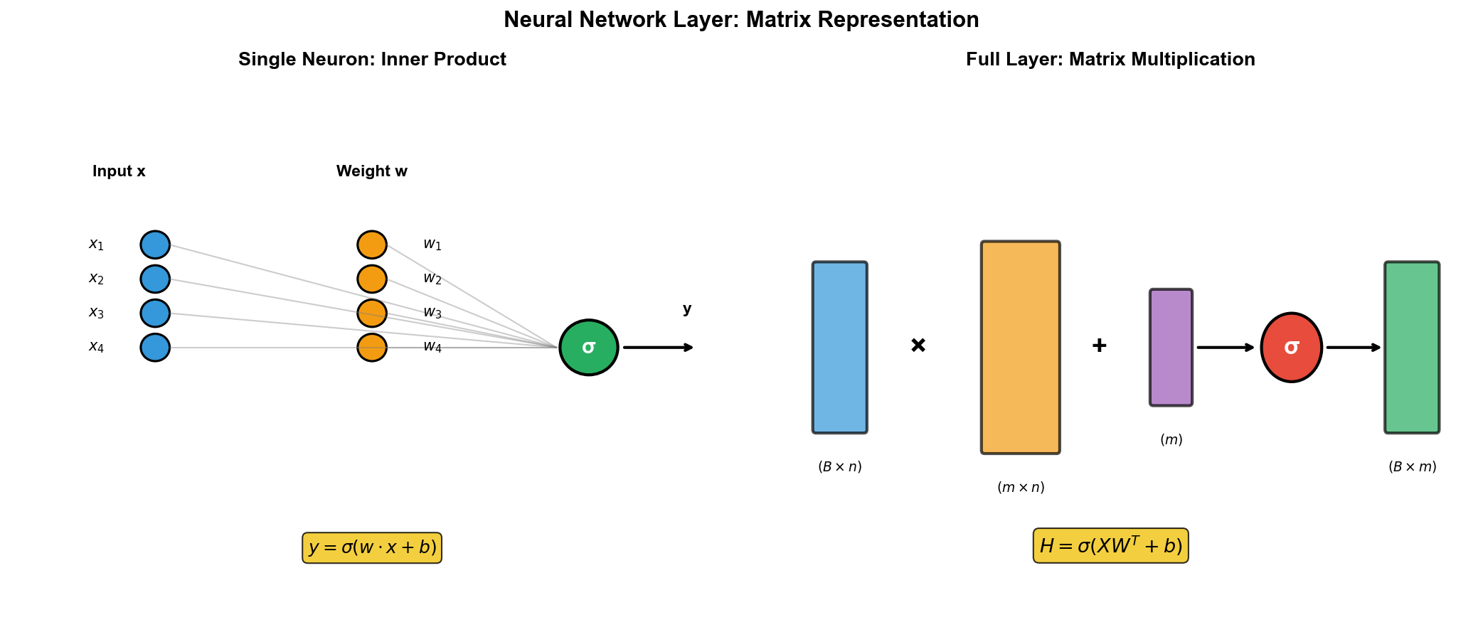
神经网络的矩阵表示
从单个神经元说起
一个神经元做的事情非常简单:接收若干输入,加权求和,加上偏置,再通过激活函数。用数学表达就是:
这个求和过程,其实就是向量的内积。如果我们把权重写成行向量
一个神经元 = 一次内积 + 一次非线性变换。就这么简单。
一层神经元的矩阵形式
现在假设一层有
这样,一层的前向传播就可以写成:
其中
直觉理解 :权重矩阵
批量处理( Batch Processing)
实际训练时,我们不会一次只处理一个样本。假设有
一层的批量前向传播变成:
这里
为什么要批量处理? 因为 GPU
擅长大规模并行计算。单个样本的计算无法充分利用 GPU
的并行能力,批量处理可以让矩阵乘法的规模变大,从而充分利用硬件。
1
2
3
4
5
6
7
8
9
10
11
12
13
14
15
16
import torchimport torch.nn as nnlinear = nn.Linear(in_features=784 , out_features=256 ) x_single = torch.randn(784 ) h_single = linear(x_single) x_batch = torch.randn(32 , 784 ) h_batch = linear(x_batch) print (f"权重矩阵形状: {linear.weight.shape} " ) print (f"偏置向量形状: {linear.bias.shape} " )
多层网络的矩阵链
多层神经网络就是多个这样的变换串联起来:
如果没有激活函数,这就是矩阵连乘
非线性的作用 :打破矩阵乘法的封闭性,使得网络能够逼近任意连续函数(万能逼近定理)。
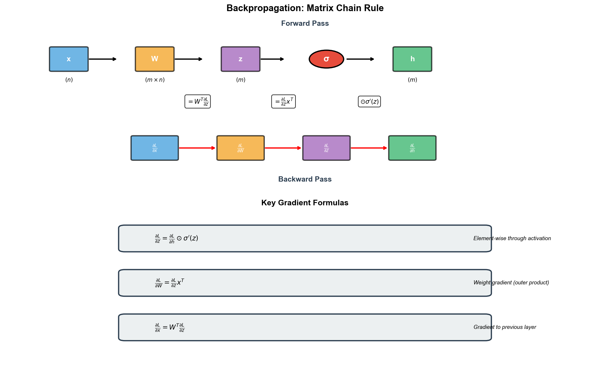
反向传播的矩阵形式
反向传播是深度学习的核心算法。从线性代数的角度看,它就是链式法则的矩阵版本。
单层的梯度
考虑一层
设
第一步 :假设我们已经知道
第二步 :通过激活函数反传。如果
其中
第三步 :计算参数梯度。这是关键的矩阵运算:
第四步 :传给前一层:
直觉理解 :
批量反向传播
对于批量数据
设
权重梯度需要对所有样本求和:
偏置梯度是对批量维度求和:
传给前一层的梯度:1 2 3 4 5 6 7 8 9 10 11 12 13 14 15 16 17 18 19 20 21 22 23 24 25 26 27 28 29 30 31 32 33 34 35 36 37 38 39 40 41 42 43 44 import torchimport torch.nn.functional as Fclass ManualLinear : def __init__ (self, in_features, out_features ): self.W = torch.randn(out_features, in_features) * (2 / (in_features + out_features)) ** 0.5 self.b = torch.zeros(out_features) self.W.requires_grad = True self.b.requires_grad = True def forward (self, x ): self.x = x self.z = x @ self.W.T + self.b self.h = F.relu(self.z) return self.h def backward (self, grad_h ): grad_z = grad_h * (self.z > 0 ).float () grad_W = grad_z.T @ self.x grad_b = grad_z.sum (dim=0 ) grad_x = grad_z @ self.W self.W.grad = grad_W self.b.grad = grad_b return grad_x layer = ManualLinear(784 , 256 ) x = torch.randn(32 , 784 ) h = layer.forward(x) grad_h = torch.randn_like(h) grad_x = layer.backward(grad_h) print (f"输入梯度形状: {grad_x.shape} " ) print (f"权重梯度形状: {layer.W.grad.shape} " )
雅可比矩阵视角
更一般地,如果
链式法则的矩阵形式就是雅可比矩阵的乘积:
对于线性层
卷积的矩阵形式
卷积神经网络(
CNN)是图像处理的核心。虽然卷积看起来和矩阵乘法不一样,但它可以转化为矩阵乘法。
一维卷积
一维离散卷积的定义:
在深度学习中,我们处理的是有限长度的信号和卷积核:
其中
矩阵形式 :一维卷积可以表示为托普利茨(
Toeplitz)矩阵乘法。假设输入
构造矩阵
则
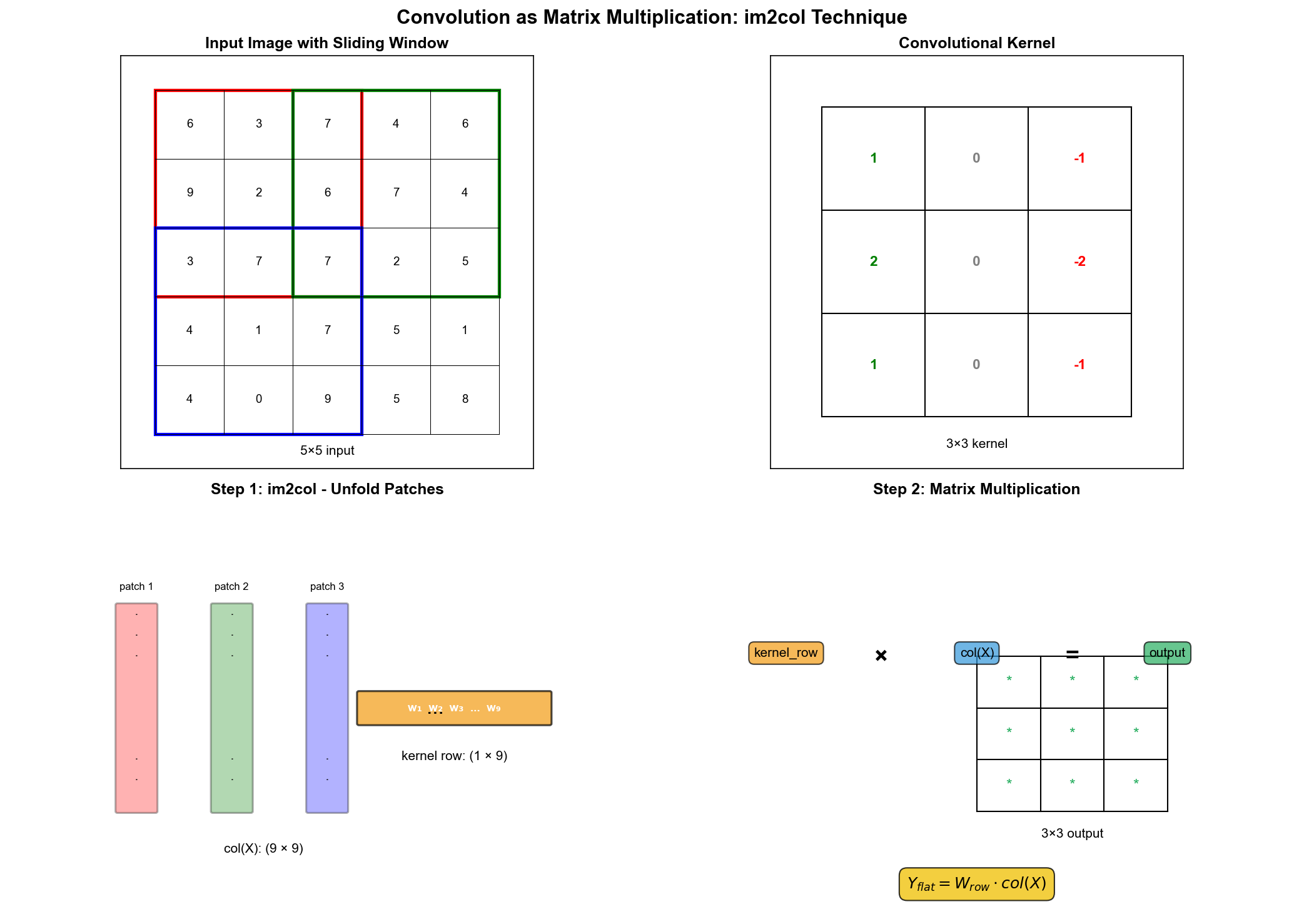
二维卷积
二维卷积用于图像处理:
im2col
技巧 :这是深度学习框架中最常用的卷积实现方法。核心思想是把卷积转化为矩阵乘法。
步骤 :
展开输入 :对于每个输出位置
展开卷积核 :将卷积核展开成一个行向量。
矩阵乘法 :
重塑输出 :将结果重塑为输出特征图的形状。
1 2 3 4 5 6 7 8 9 10 11 12 13 14 15 16 17 18 19 20 21 22 23 24 25 26 27 28 29 30 31 32 33 34 35 36 37 38 39 40 41 42 43 44 45 46 47 48 49 50 51 52 53 54 55 56 57 58 59 60 61 62 63 import torchimport torch.nn.functional as Fdef im2col_naive (x, kernel_size, stride=1 , padding=0 ): """ 将输入图像转换为列矩阵 x: (batch, channels, height, width) """ batch, channels, h, w = x.shape kh, kw = kernel_size if padding > 0 : x = F.pad(x, [padding] * 4 ) _, _, h_pad, w_pad = x.shape out_h = (h_pad - kh) // stride + 1 out_w = (w_pad - kw) // stride + 1 col = torch.zeros(batch, channels * kh * kw, out_h * out_w) for i in range (out_h): for j in range (out_w): patch = x[:, :, i*stride:i*stride+kh, j*stride:j*stride+kw] col[:, :, i*out_w+j] = patch.reshape(batch, -1 ) return col, out_h, out_w def conv2d_via_im2col (x, weight, stride=1 , padding=0 ): """ 使用 im2col 实现 2D 卷积 x: (batch, in_channels, h, w) weight: (out_channels, in_channels, kh, kw) """ batch = x.shape[0 ] out_channels, in_channels, kh, kw = weight.shape col, out_h, out_w = im2col_naive(x, (kh, kw), stride, padding) weight_col = weight.reshape(out_channels, -1 ) out = weight_col @ col out = out.reshape(batch, out_channels, out_h, out_w) return out x = torch.randn(2 , 3 , 8 , 8 ) weight = torch.randn(16 , 3 , 3 , 3 ) y1 = conv2d_via_im2col(x, weight, padding=1 ) y2 = F.conv2d(x, weight, padding=1 ) print (f"差异: {(y1 - y2).abs ().max ().item():.6 f} " )
为什么用 im2col? 因为 GEMM(通用矩阵乘法)在 CPU 和
GPU 上都有高度优化的实现(如 cuBLAS)。虽然 im2col
会增加内存使用(输入被复制多次),但利用高效的 GEMM
带来的速度提升通常远超内存的开销。
转置卷积(反卷积)
转置卷积用于上采样,常见于生成模型和语义分割的解码器。
直觉 :如果正向卷积将
矩阵视角 :如果正向卷积可以表示为
注意:转置卷积不是 卷积的逆运算。
1 2 3 4 5 6 7 8 9 10 11 conv = nn.Conv2d(3 , 16 , kernel_size=3 , stride=2 , padding=1 ) conv_transpose = nn.ConvTranspose2d(16 , 3 , kernel_size=3 , stride=2 , padding=1 , output_padding=1 ) x = torch.randn(1 , 3 , 32 , 32 ) y = conv(x) x_reconstructed = conv_transpose(y) print (f"输入形状: {x.shape} " )print (f"卷积后形状: {y.shape} " )print (f"转置卷积后形状: {x_reconstructed.shape} " )
深度可分离卷积
标准卷积的参数量是
深度卷积(
Depthwise) :每个输入通道独立卷积,不混合通道。参数量:
逐点卷积( Pointwise) :
总参数量:
矩阵视角 :这是一种低秩分解。标准卷积的权重张量可以近似分解为深度和逐点两部分的乘积。
1 2 3 4 5 6 7 8 9 10 11 12 13 14 15 16 17 18 19 20 21 22 23 24 class DepthwiseSeparableConv (nn.Module): def __init__ (self, in_channels, out_channels, kernel_size, stride=1 , padding=0 ): super ().__init__() self.depthwise = nn.Conv2d(in_channels, in_channels, kernel_size, stride=stride, padding=padding, groups=in_channels) self.pointwise = nn.Conv2d(in_channels, out_channels, kernel_size=1 ) def forward (self, x ): x = self.depthwise(x) x = self.pointwise(x) return x standard_conv = nn.Conv2d(64 , 128 , 3 , padding=1 ) depthwise_sep = DepthwiseSeparableConv(64 , 128 , 3 , padding=1 ) print (f"标准卷积参数量: {sum (p.numel() for p in standard_conv.parameters())} " )print (f"深度可分离卷积参数量: {sum (p.numel() for p in depthwise_sep.parameters())} " )
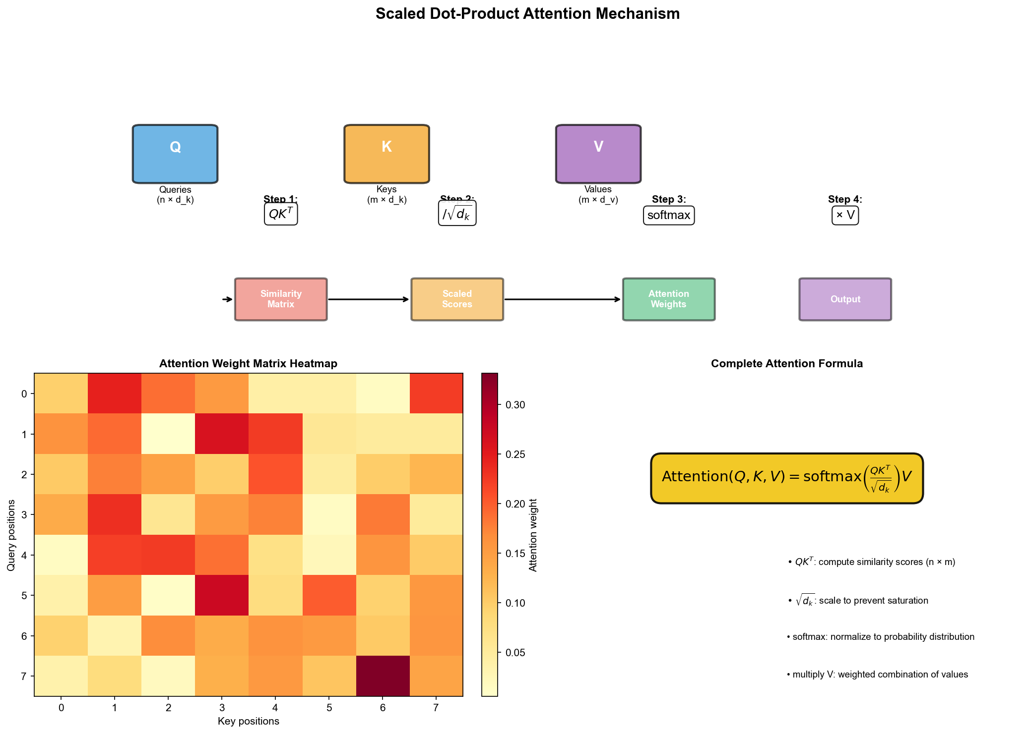
Attention 机制中的矩阵运算
Attention
是现代深度学习最重要的创新之一。它的核心完全建立在矩阵运算之上。
注意力的直觉
想象你在图书馆找资料。你有一个问题( Query),图书馆有很多书(
Key-Value 对)。你先用问题和每本书的关键词(
Key)比对相关性,然后根据相关性加权获取书的内容( Value)。
Attention 做的事情 :给定查询
缩放点积注意力
让我们拆解这个公式:
第一步 :
假设
第二步 :除以
为什么要缩放?假设
第三步 : softmax ——归一化
对每一行(每个查询)做 softmax,得到注意力权重。权重和为
1,可以解释为概率分布。
第四步 :乘以
假设
每个输出是所有值向量的加权平均,权重由注意力决定。
1
2
3
4
5
6
7
8
9
10
11
12
13
14
15
16
17
18
19
20
21
22
23
24
25
26
27
28
29
30
31
32
33
34
35
36
37
38
39
40
41
import torchimport torch.nn.functional as Fimport mathdef scaled_dot_product_attention (Q, K, V, mask=None ): """ 缩放点积注意力 Q: (batch, n_heads, seq_len_q, d_k) K: (batch, n_heads, seq_len_k, d_k) V: (batch, n_heads, seq_len_k, d_v) mask: (batch, 1, 1, seq_len_k) 或 (batch, 1, seq_len_q, seq_len_k) """ d_k = Q.size(-1 ) scores = torch.matmul(Q, K.transpose(-2 , -1 )) / math.sqrt(d_k) if mask is not None : scores = scores.masked_fill(mask == 0 , float ('-inf' )) attn_weights = F.softmax(scores, dim=-1 ) output = torch.matmul(attn_weights, V) return output, attn_weights batch, n_heads, seq_len, d_k = 2 , 8 , 10 , 64 Q = torch.randn(batch, n_heads, seq_len, d_k) K = torch.randn(batch, n_heads, seq_len, d_k) V = torch.randn(batch, n_heads, seq_len, d_k) output, weights = scaled_dot_product_attention(Q, K, V) print (f"输出形状: {output.shape} " ) print (f"注意力权重形状: {weights.shape} " ) print (f"权重每行和: {weights[0 , 0 , 0 ].sum ().item():.4 f} " )
多头注意力
单一注意力只能学习一种"关注模式"。多头注意力让模型同时学习多种不同的关注模式。
其中每个头:
线性代数视角 :
-
参数形状 : - 输入维度1 2 3 4 5 6 7 8 9 10 11 12 13 14 15 16 17 18 19 20 21 22 23 24 25 26 27 28 29 30 31 32 33 34 35 36 37 38 39 40 41 class MultiHeadAttention (nn.Module): def __init__ (self, d_model, n_heads ): super ().__init__() assert d_model % n_heads == 0 self.d_model = d_model self.n_heads = n_heads self.d_k = d_model // n_heads self.W_q = nn.Linear(d_model, d_model) self.W_k = nn.Linear(d_model, d_model) self.W_v = nn.Linear(d_model, d_model) self.W_o = nn.Linear(d_model, d_model) def forward (self, Q, K, V, mask=None ): batch_size = Q.size(0 ) Q = self.W_q(Q).view(batch_size, -1 , self.n_heads, self.d_k).transpose(1 , 2 ) K = self.W_k(K).view(batch_size, -1 , self.n_heads, self.d_k).transpose(1 , 2 ) V = self.W_v(V).view(batch_size, -1 , self.n_heads, self.d_k).transpose(1 , 2 ) attn_output, attn_weights = scaled_dot_product_attention(Q, K, V, mask) attn_output = attn_output.transpose(1 , 2 ).contiguous().view(batch_size, -1 , self.d_model) output = self.W_o(attn_output) return output, attn_weights mha = MultiHeadAttention(d_model=512 , n_heads=8 ) x = torch.randn(2 , 10 , 512 ) output, weights = mha(x, x, x) print (f"输出形状: {output.shape} " )
注意力的计算复杂度
标准注意力的时间和空间复杂度都是
对于长序列,这是主要瓶颈。各种高效注意力变体( Sparse Attention,
Linear Attention, FlashAttention 等)都是为了解决这个问题。
FlashAttention 是一种算法优化,通过分块计算和减少
GPU 内存访问来加速标准注意力,不改变数学结果。
Transformer 是现代 NLP 和多模态 AI
的基础架构。让我们从线性代数的角度完整解读它。
一个 Encoder 层包含:
多头自注意力 (已介绍)前馈网络( FFN) :两层全连接 + 激活函数残差连接 层归一化
前馈网络 :
通常
直觉 : FFN
是逐位置的——对序列中每个位置独立应用相同的变换。它可以看作是一个两层的小型
MLP,先扩展维度、引入非线性,再压缩回原维度。
残差连接 :
残差连接让梯度可以"跳过"复杂的变换直接传回去,缓解梯度消失问题。
Decoder 比 Encoder 多一个交叉注意力 (
Cross-Attention):
Query 来自 Decoder 的上一层输出
Key 和 Value 来自 Encoder 的输出
这让 Decoder 能够"看到"Encoder 处理的输入。
另外, Decoder 的自注意力是因果的 (
Causal):位置
被 mask 的位置在 softmax 前被设为
1 2 3 4 5 6 7 8 9 10 11 12 def create_causal_mask (seq_len ): """创建因果注意力 mask""" mask = torch.tril(torch.ones(seq_len, seq_len)) return mask.unsqueeze(0 ).unsqueeze(0 ) mask = create_causal_mask(5 ) print (mask[0 , 0 ])
位置编码
Transformer 没有循环结构,自注意力对位置是不敏感的( permutation
equivariant)。位置编码给模型提供位置信息。
正弦位置编码 :
线性代数视角 :每个位置被编码为一个
1 2 3 4 5 6 7 8 9 10 11 12 13 14 15 16 17 class PositionalEncoding (nn.Module): def __init__ (self, d_model, max_len=5000 ): super ().__init__() pe = torch.zeros(max_len, d_model) position = torch.arange(0 , max_len, dtype=torch.float ).unsqueeze(1 ) div_term = torch.exp(torch.arange(0 , d_model, 2 ).float () * (-math.log(10000.0 ) / d_model)) pe[:, 0 ::2 ] = torch.sin(position * div_term) pe[:, 1 ::2 ] = torch.cos(position * div_term) pe = pe.unsqueeze(0 ) self.register_buffer('pe' , pe) def forward (self, x ): return x + self.pe[:, :x.size(1 ), :]
1 2 3 4 5 6 7 8 9 10 11 12 13 14 15 16 17 18 19 20 21 22 23 24 25 26 class TransformerEncoderLayer (nn.Module): def __init__ (self, d_model, n_heads, d_ff, dropout=0.1 ): super ().__init__() self.self_attn = MultiHeadAttention(d_model, n_heads) self.ffn = nn.Sequential( nn.Linear(d_model, d_ff), nn.ReLU(), nn.Dropout(dropout), nn.Linear(d_ff, d_model) ) self.norm1 = nn.LayerNorm(d_model) self.norm2 = nn.LayerNorm(d_model) self.dropout = nn.Dropout(dropout) def forward (self, x, mask=None ): attn_output, _ = self.self_attn(x, x, x, mask) x = self.norm1(x + self.dropout(attn_output)) ffn_output = self.ffn(x) x = self.norm2(x + self.dropout(ffn_output)) return x
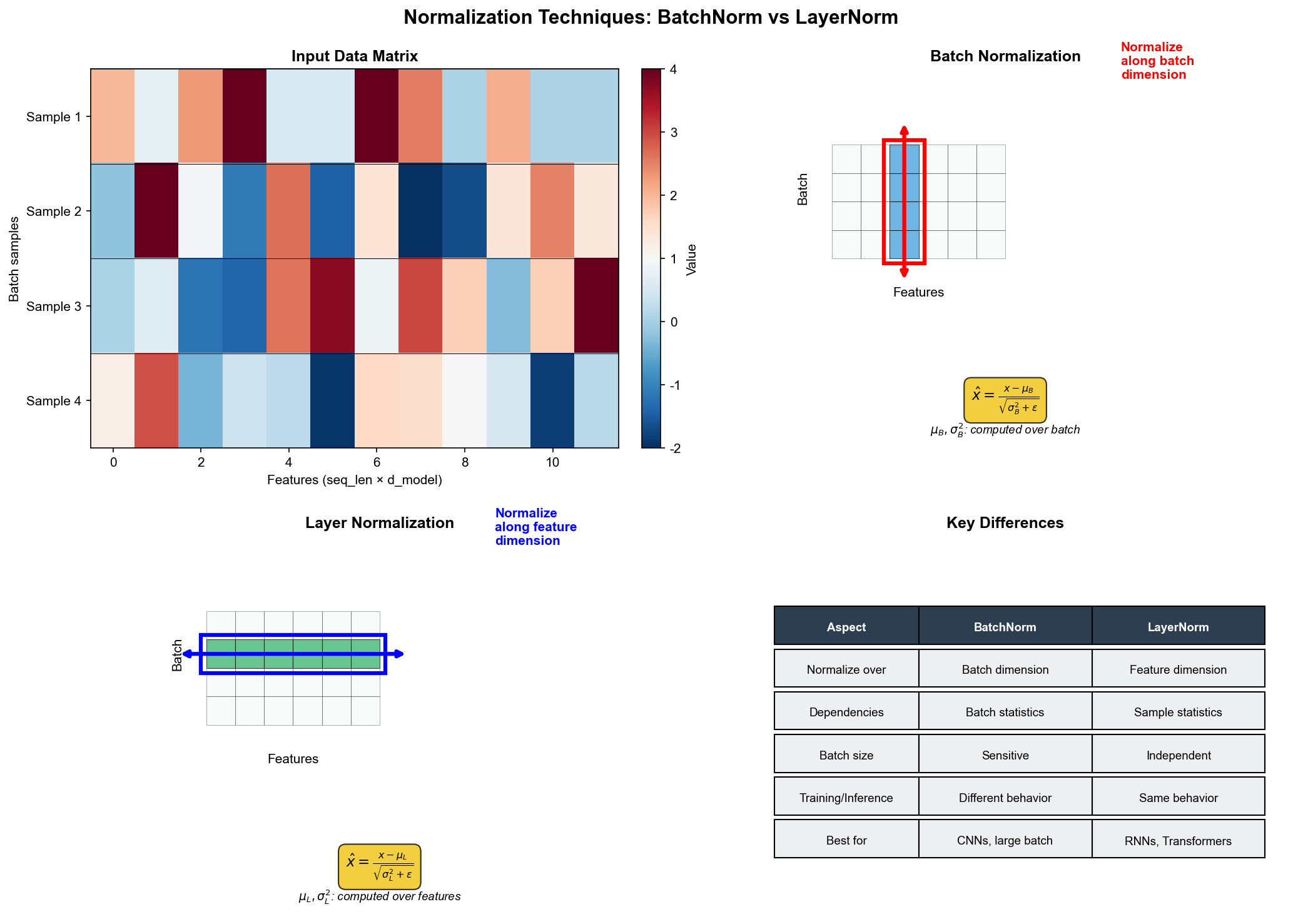
BatchNorm 和 LayerNorm
归一化层是深度学习中的关键组件。它们通过标准化激活值来稳定训练。
Batch Normalization
操作 :对每个特征,在 batch
维度上计算均值和方差,然后标准化:
其中
标准化后,再用可学习参数缩放和平移:
输入形状 :对于卷积层
问题 : BN 依赖 batch 统计量。小 batch
时估计不准;推理时需要用训练时积累的移动平均。
1 2 3 4 5 6 7 8 9 10 11 12 13 14 15 16 17 18 19 20 21 22 23 24 25 26 27 28 29 class BatchNorm1d (nn.Module): def __init__ (self, num_features, eps=1e-5 , momentum=0.1 ): super ().__init__() self.eps = eps self.momentum = momentum self.gamma = nn.Parameter(torch.ones(num_features)) self.beta = nn.Parameter(torch.zeros(num_features)) self.register_buffer('running_mean' , torch.zeros(num_features)) self.register_buffer('running_var' , torch.ones(num_features)) def forward (self, x ): if self.training: mean = x.mean(dim=0 ) var = x.var(dim=0 , unbiased=False ) self.running_mean = (1 - self.momentum) * self.running_mean + self.momentum * mean self.running_var = (1 - self.momentum) * self.running_var + self.momentum * var else : mean = self.running_mean var = self.running_var x_norm = (x - mean) / torch.sqrt(var + self.eps) return self.gamma * x_norm + self.beta
Layer Normalization
操作 :对每个样本,在特征维度上计算均值和方差:
其中同一个样本的所有特征 上计算的。
输入形状 :对于
优点 :不依赖 batch,适合小 batch 和序列模型( RNN 、
Transformer)。
矩阵视角的区别 :
BatchNorm :沿着 batch
维度(矩阵的行)标准化每个特征(列)LayerNorm :沿着特征维度(矩阵的列)标准化每个样本(行)
1 2 3 4 5 6 7 8 9 10 11 12 13 14 15 16 17 18 19 20 21 22 23 24 25 26 27 28 29 30 31 class LayerNorm (nn.Module): def __init__ (self, normalized_shape, eps=1e-5 ): super ().__init__() self.eps = eps self.gamma = nn.Parameter(torch.ones(normalized_shape)) self.beta = nn.Parameter(torch.zeros(normalized_shape)) def forward (self, x ): mean = x.mean(dim=-1 , keepdim=True ) var = x.var(dim=-1 , keepdim=True , unbiased=False ) x_norm = (x - mean) / torch.sqrt(var + self.eps) return self.gamma * x_norm + self.beta x = torch.randn(32 , 10 , 512 ) bn = nn.BatchNorm1d(512 ) ln = nn.LayerNorm(512 ) x_bn = bn(x.transpose(1 , 2 )).transpose(1 , 2 ) x_ln = ln(x) print (f"BN 输出形状: {x_bn.shape} " ) print (f"LN 输出形状: {x_ln.shape} " )
RMSNorm
RMSNorm 是 LayerNorm 的简化版,只用均方根(
RMS)标准化,不减均值:
优点 :计算更简单,效果相近。 LLaMA 等模型使用
RMSNorm 。
1 2 3 4 5 6 7 8 9 class RMSNorm (nn.Module): def __init__ (self, dim, eps=1e-6 ): super ().__init__() self.eps = eps self.weight = nn.Parameter(torch.ones(dim)) def forward (self, x ): rms = torch.sqrt(x.pow (2 ).mean(dim=-1 , keepdim=True ) + self.eps) return self.weight * x / rms
参数高效微调: LoRA
大语言模型( LLM)有数十亿参数,全量微调成本很高。 LoRA( Low-Rank
Adaptation)是一种高效的微调方法,其核心是低秩矩阵分解。
核心思想
预训练模型的权重为
其中
参数量对比 : - 全量微调:
例如,对于
为什么低秩有效?
研究表明,预训练模型在微调时的权重变化具有低秩结构。也就是说,
直觉 :微调是在预训练模型学到的特征空间上做小调整,不需要改变整个空间的结构。低秩更新只调整一个低维子空间。
实现
1 2 3 4 5 6 7 8 9 10 11 12 13 14 15 16 17 18 19 20 21 22 23 24 25 26 27 28 29 30 31 32 33 34 35 36 37 38 39 40 41 42 43 44 45 46 47 48 49 50 51 52 53 class LoRALinear (nn.Module): def __init__ (self, base_layer, r=8 , alpha=16 , dropout=0.1 ): """ base_layer: 原始的 nn.Linear 层 r: LoRA 的秩 alpha: 缩放因子 """ super ().__init__() self.base_layer = base_layer self.r = r self.alpha = alpha in_features = base_layer.in_features out_features = base_layer.out_features self.lora_A = nn.Parameter(torch.randn(r, in_features) * 0.01 ) self.lora_B = nn.Parameter(torch.zeros(out_features, r)) self.scaling = alpha / r self.dropout = nn.Dropout(dropout) for param in base_layer.parameters(): param.requires_grad = False def forward (self, x ): base_output = self.base_layer(x) lora_output = self.dropout(x) @ self.lora_A.T @ self.lora_B.T * self.scaling return base_output + lora_output def merge_weights (self ): """将 LoRA 权重合并到原始权重,推理时使用""" self.base_layer.weight.data += (self.lora_B @ self.lora_A) * self.scaling base = nn.Linear(4096 , 4096 ) lora = LoRALinear(base, r=8 ) print (f"原始参数量: {sum (p.numel() for p in base.parameters())} " ) print (f"LoRA 可训练参数量: {sum (p.numel() for p in lora.parameters() if p.requires_grad)} " ) x = torch.randn(2 , 10 , 4096 ) y = lora(x) print (f"输出形状: {y.shape} " )
通常对注意力层的
1 2 3 4 5 6 7 8 9 10 11 12 13 14 15 16 17 def apply_lora_to_attention (attention_module, r=8 , alpha=16 ): """给 MultiHeadAttention 添加 LoRA""" attention_module.W_q = LoRALinear(attention_module.W_q, r=r, alpha=alpha) attention_module.W_k = LoRALinear(attention_module.W_k, r=r, alpha=alpha) attention_module.W_v = LoRALinear(attention_module.W_v, r=r, alpha=alpha) attention_module.W_o = LoRALinear(attention_module.W_o, r=r, alpha=alpha) return attention_module mha = MultiHeadAttention(d_model=512 , n_heads=8 ) mha_with_lora = apply_lora_to_attention(mha, r=8 ) total_params = sum (p.numel() for p in mha_with_lora.parameters()) trainable_params = sum (p.numel() for p in mha_with_lora.parameters() if p.requires_grad) print (f"总参数量: {total_params} " )print (f"可训练参数量: {trainable_params} " )print (f"可训练比例: {trainable_params / total_params * 100 :.2 f} %" )
QLoRA 和其他变体
QLoRA :结合量化和 LoRA 。基础模型用 4 位量化存储,
LoRA 参数用 FP16/BF16,进一步减少内存。
DoRA :将权重分解为方向和幅度两部分,分别用 LoRA
适配,效果更好。
AdaLoRA :自适应分配不同层的秩
深度学习优化中的线性代数
权重初始化
好的初始化对训练至关重要。目标是让前向传播和反向传播时信号不会爆炸或消失。
Xavier 初始化 (适用于 tanh/sigmoid):
或者高斯版本:
推导思路 :假设输入
He 初始化 (适用于 ReLU):
1 2 3 4 5 6 7 8 9 10 11 12 13 14 15 16 17 18 def xavier_init (shape ): n_in, n_out = shape std = (2 / (n_in + n_out)) ** 0.5 return torch.randn(shape) * std def he_init (shape ): n_in, n_out = shape std = (2 / n_in) ** 0.5 return torch.randn(shape) * std n_in, n_out = 1000 , 1000 W = he_init((n_out, n_in)) x = torch.randn(100 , n_in) y = x @ W.T print (f"输入方差: {x.var().item():.4 f} " )print (f"输出方差: {y.var().item():.4 f} " )
梯度问题与奇异值
深层网络中,梯度需要经过很多层传播。如果每层的雅可比矩阵的奇异值都大于
1,梯度会爆炸;都小于 1,梯度会消失。
设网络为
梯度的范数大致是各层雅可比矩阵奇异值的乘积。
解决方案 :
残差连接 :归一化 :控制激活值的范围梯度裁剪 :
优化器的矩阵视角
SGD :梯度下降
SGD with Momentum :累积梯度
Adam :自适应学习率
线性代数视角 : Adam 相当于用对角预条件矩阵
练习题
基础题
1. 证明:对于线性层
2. 假设输入
3. 解释为什么多头注意力中,每个头的维度通常设为
4. BatchNorm 和 LayerNorm
分别在哪些维度上计算均值和方差?对于形状为
进阶题
5. 推导缩放点积注意力中除以
6. 对于 im2col 方法: - 假设输入
7. 证明:如果
8. 分析 ResNet 残差块
编程题
9. 实现一个完整的 Transformer
Encoder(包含多层),并用它处理一个简单的序列分类任务。
1 2 3 4 5 6 7 8 9 10 11 12 13 14 15 16 class TransformerEncoder (nn.Module): def __init__ (self, d_model, n_heads, d_ff, n_layers, dropout=0.1 ): super ().__init__() pass def forward (self, x, mask=None ): pass encoder = TransformerEncoder(d_model=256 , n_heads=4 , d_ff=1024 , n_layers=4 ) x = torch.randn(2 , 20 , 256 ) output = encoder(x) print (f"输出形状: {output.shape} " )
10. 实现一个简化的 LoRA 训练流程: -
加载一个预训练的小型模型(如一个简单的分类器) - 对其线性层应用 LoRA -
在新任务上微调 LoRA 参数 - 比较全量微调和 LoRA 微调的参数量和效果
11. 实现并可视化不同归一化方法的效果: -
生成一个随机 batch - 分别应用 BatchNorm 、 LayerNorm 、 RMSNorm -
可视化归一化前后特征分布的变化
12. 分析一个实际的 Transformer 模型(如 BERT-tiny 或
GPT-2-small)的计算复杂度: - 统计不同组件(注意力、 FFN 、归一化等)的
FLOPs 占比 - 分析序列长度对计算量的影响 -
绘制计算量随序列长度变化的曲线
思考题
13. 为什么 Transformer 中普遍使用 LayerNorm 而不是
BatchNorm?从训练稳定性、序列长度变化、并行计算等角度分析。
14. LoRA
假设微调时的权重变化是低秩的。在什么情况下这个假设可能不成立?如何检测?
15. 如果要将传统的 2D CNN 迁移到处理 3D
数据(如视频或医学影像),从矩阵运算的角度分析计算量会如何变化。
本章总结
深度学习的核心操作都可以用线性代数来描述:
全连接层 :矩阵乘法 + 非线性激活反向传播 :链式法则的矩阵形式,梯度通过转置矩阵传播卷积 :可以通过 im2col 转化为矩阵乘法,利用高效 GEMM
加速注意力机制 :查询-键点积计算相似度,对值加权求和Transformer :注意力 + FFN + 残差 +
归一化的组合归一化层 :在不同维度上标准化,稳定训练LoRA :低秩矩阵分解实现高效微调
理解这些线性代数基础,能让你: 1. 更好地理解模型的工作原理 2.
高效地实现和优化模型 3. 设计新的网络架构 4.
调试训练中的问题(梯度消失/爆炸等)
参考资料
Vaswani, A., et al. "Attention is All You Need." NeurIPS 2017.
Hu, E., et al. "LoRA: Low-Rank Adaptation of Large Language Models."
ICLR 2022.
Ba, J., Kiros, J., & Hinton, G. "Layer Normalization." arXiv
2016.
Ioffe, S., & Szegedy, C. "Batch Normalization." ICML 2015.
He, K., et al. "Deep Residual Learning for Image Recognition." CVPR
2016.
Glorot,
X., & Bengio, Y. "Understanding the difficulty of training deep
feedforward neural networks." AISTATS 2010.
本文是《线性代数的本质与应用》系列的第十六章,共 18 章。