机器学习数学推导（十二） XGBoost 与 LightGBM

XGBoost 和 LightGBM 是工业界最流行的梯度提升框架——它们在 GBDT 基础上引入精妙的数学优化与工程创新，实现了精度与效率的完美平衡。从 XGBoost 的二阶优化到 LightGBM 的直方图加速，从正则化惩罚到梯度单边采样，这些技术背后蕴含深刻的数学洞察。本章将系统推导 XGBoost 和 LightGBM 的数学原理、算法细节与实战技巧。

XGBoost：极致优化的梯度提升

正则化目标函数

标准 GBDT 最小化损失：

XGBoost 目标：添加树复杂度正则化

其中： - i^{(t)} = {k=1}^t f_k(_i) $是前$ t $轮的预测$ f_t $是第$ t $棵树$ 是正则化项

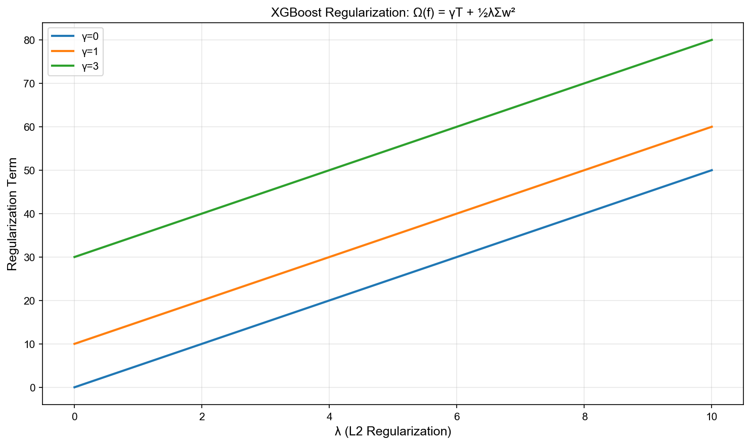
树的正则化：

其中： - 是叶节点数 - 是叶节点的权重（预测值） - $惩罚叶节点数（类似剪枝）$ 惩罚叶权重（正则化）

二阶泰勒展开

在_i^{(t-1)}$ 处对损失函数做二阶泰勒展开：

L(y_i, _i^{(t-1)} + f_t(_i)) L(y_i, _i^{(t-1)}) + g_i f_t(_i) + h_i f_t^2(_i) $$

其中： - 是一阶梯度 - 是二阶梯度（ Hessian）

目标函数简化：

（省略常数项_i L(y_i, _i^{(t-1)})$）

树结构下的目标函数

树的表示：第棵树定义为

f_t() = w_{q()} $$

其中是将样本映射到叶节点的函数，是叶节点的权重。

重新组织目标：将样本按叶节点分组

其中是叶节点包含的样本集。

最优叶权重：对求导并令为 0

w_j^{*} = - = - $$

其中，。

代入最优权重：

这是给定树结构下的最优损失。

分裂增益计算

问题：如何选择最优分裂点？

对于叶节点$ j $，考虑在特征$ k $的阈值$ 处分裂： - 左子节点： - 右子节点：

分裂前的损失：

分裂后的损失：

分裂增益（ Gain）：

分裂准则： - 若 > 0 $，执行分裂选择$ 最大的特征和阈值

常用损失函数的梯度

平方损失（回归）

L(y, ) = (y - )^2

g_i = _i - y_i, h_i = 1 $$

Logistic 损失（二分类）

L(y, ) = y (1 + e^{-} ) + (1 - y) (1 + e^{} ) $$

令，则：

g_i = p_i - y_i, h_i = p_i (1 - p_i) $$

Softmax 损失（多分类）

对于类别：

g_{ik} = p_{ik} - (y_i = k), h_{ik} = 2 p_{ik} (1 - p_{ik}) $$

其中。

分裂算法

精确贪心算法

输入：当前节点的样本集$I $，特征集$

算法： 1. 初始化：{} = 0$，{} = $枚举特征：对每个特征$ k $：对$ I $中的样本按特征$ k$ 排序 - 枚举阈值：对每个可能的分裂点 $：计算$ G L, H_L, G_R, H_R $计算$ - 若 > {} $，更新最优分裂返回：最优分裂$ (k^, ^)$

复杂度：，是分裂点数，是特征数。

近似算法（分位数 sketch）

精确算法在大数据上不可行。近似算法：用分位数代替所有可能阈值。

分位数候选生成： - 全局：在树构建前，一次性计算所有特征的分位数（如） - 局部：每次分裂时，重新计算当前节点的分位数

加权分位数：考虑二阶梯度作为样本权重

r_k() = $$

寻找候选分裂点{{k1}, , {kl}} $ 使得。

稀疏感知算法

问题：现实数据常含缺失值或稀疏特征（如 one-hot 编码）。

默认方向：为每个节点学习默认分裂方向（左或右）。

算法： 1. 将非缺失样本分别尝试分到左、右子节点 2. 缺失样本分到默认方向 3. 选择增益最大的分裂和默认方向

实现：只遍历非缺失值，。

LightGBM：高效梯度提升

Histogram 算法

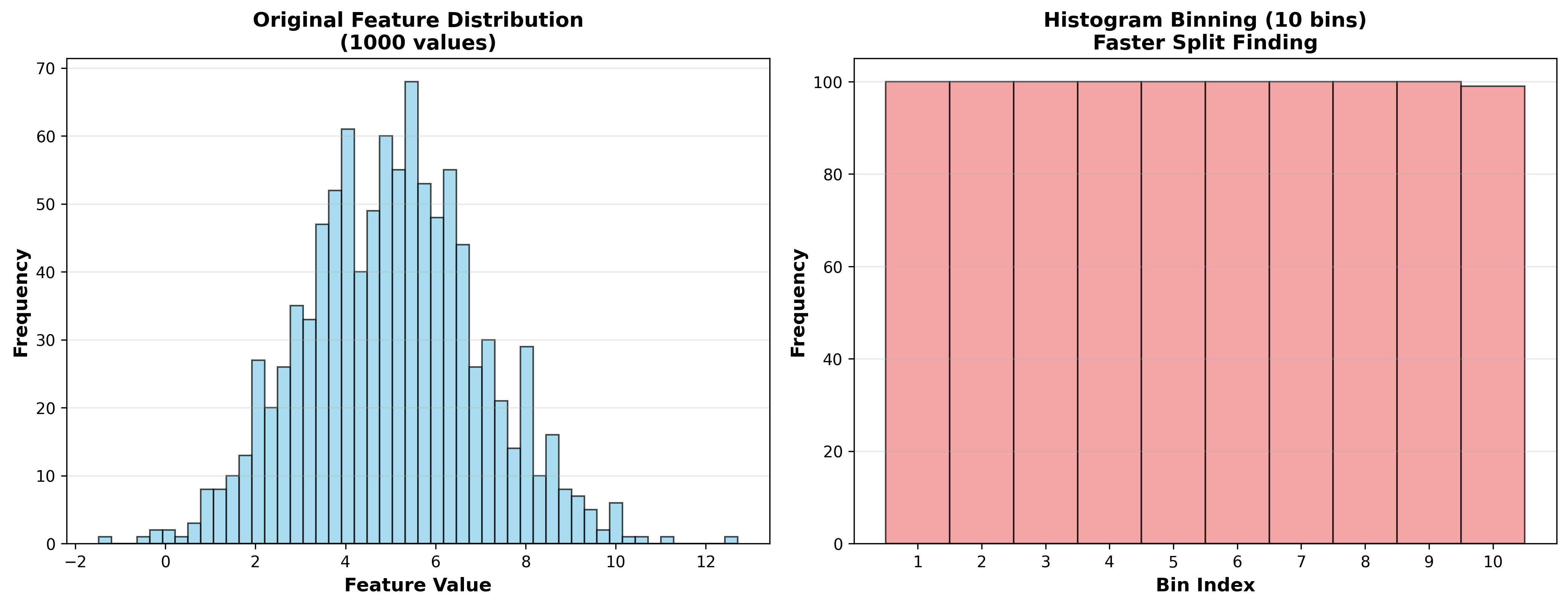
核心思想：将连续特征离散化为个桶（ bins），用直方图统计梯度。

优势： - 内存：存储直方图而非原始数据，而非 - 计算：遍历个桶而非个样本，而非 - 通信：分布式训练中，传输直方图而非数据

算法： 1. 特征离散化：将特征映射到{0, 1, , k-1} $构建直方图：对每个桶$ b$，累积梯度和 Hessian

G_b = {i: (x_i^{(k)}) = b} g_i, H_b = {i: (x_i^{(k)}) = b} h_i

遍历桶：计算每个桶的分裂增益（而非）

Histogram 差分：对于兄弟节点，只需计算一个直方图，另一个通过父节点减法得到：

减少一半计算量。

Leaf-wise 生长策略

Level-wise（ XGBoost）：每次分裂所有叶节点（同一层）

Leaf-wise（ LightGBM）：每次分裂增益最大的单个叶节点

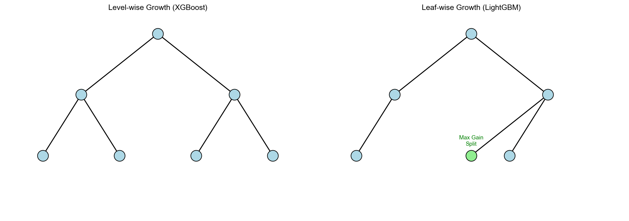
优势： - 更高的精度（优先分裂最有价值的节点） - 更快的收敛（不浪费计算在低增益节点）

风险： - 易过拟合（树更深更不平衡） - 需要 max_depth 限制

GOSS：梯度单边采样

动机：不同样本对梯度的贡献不同，梯度大的样本更重要。

算法： 1. 排序：按梯度绝对值降序排列样本 2. 采样： - 保留前的大梯度样本（如$ a=0.2 $）从剩余样本随机采样$ b % $（如$ b=0.2 $）重加权：小梯度样本乘以$ 以补偿采样

分裂增益估计：

其中是大梯度样本集，是采样的小梯度样本集。

理论保证： GOSS 的估计误差有界（证明见 LightGBM 论文）。

EFB：互斥特征绑定

动机：稀疏特征间互斥（如 one-hot 编码），可绑定为单个特征。

问题形式：将个特征分组，使每组内特征尽可能互斥，最小化组数。

这是图着色问题（ NP-hard）。

近似算法： 1. 构造冲突图：节点为特征，边权重为特征间冲突度（非零值同时出现的次数） 2. 贪心着色：按冲突度降序，依次分配特征到组（冲突度最小的组）

特征绑定：将组内特征合并，通过偏移避免冲突：

其中_i $是前$ i-1$ 个特征的桶数之和。

示例：特征 A（ 3 个桶）、特征 B（ 5 个桶）绑定后： - A 的桶 0, 1, 2 映射到 0, 1, 2 - B 的桶 0, 1, 2, 3, 4 映射到 3, 4, 5, 6, 7

总共 8 个桶。

XGBoost vs LightGBM 对比

维度	XGBoost	LightGBM
分裂策略	Level-wise	Leaf-wise
基本算法	预排序	Histogram
采样	行列采样	GOSS + EFB
内存	高（存储排序后数据）	低（直方图）
速度	中等	快
精度	高	高
过拟合风险	低	高（需调参）
稀疏特征	稀疏感知	EFB 优化
分布式	支持	支持（更高效）

完整实现（简化版）

import numpy as np

class XGBoostTree:
    """XGBoost 单棵树（简化版）"""
    def __init__(self, max_depth=6, min_child_weight=1, gamma=0, lambda_=1):
        self.max_depth = max_depth
        self.min_child_weight = min_child_weight
        self.gamma = gamma
        self.lambda_ = lambda_
        self.tree = None
        
    def fit(self, X, g, h):
        """
        参数:
            X: 特征矩阵
            g: 一阶梯度
            h: 二阶梯度
        """
        self.tree = self._build_tree(X, g, h, depth=0)
        return self
    
    def _calc_gain(self, G_L, H_L, G_R, H_R, G, H):
        """计算分裂增益"""
        gain = 0.5 * (
            G_L ** 2 / (H_L + self.lambda_) +
            G_R ** 2 / (H_R + self.lambda_) -
            G ** 2 / (H + self.lambda_)
        ) - self.gamma
        return gain
    
    def _find_best_split(self, X, g, h):
        """寻找最优分裂"""
        N, d = X.shape
        best_gain = 0
        best_split = None
        
        G = np.sum(g)
        H = np.sum(h)
        
        for j in range(d):
            # 按特征 j 排序
            sorted_idx = np.argsort(X[:, j])
            X_sorted = X[sorted_idx, j]
            g_sorted = g[sorted_idx]
            h_sorted = h[sorted_idx]
            
            G_L, H_L = 0, 0
            G_R, H_R = G, H
            
            for i in range(N - 1):
                G_L += g_sorted[i]
                H_L += h_sorted[i]
                G_R -= g_sorted[i]
                H_R -= h_sorted[i]
                
                # 跳过相同值
                if X_sorted[i] == X_sorted[i + 1]:
                    continue
                
                # 检查最小 Hessian 和约束
                if H_L < self.min_child_weight or H_R < self.min_child_weight:
                    continue
                
                gain = self._calc_gain(G_L, H_L, G_R, H_R, G, H)
                
                if gain > best_gain:
                    best_gain = gain
                    threshold = (X_sorted[i] + X_sorted[i + 1]) / 2
                    best_split = (j, threshold, G_L, H_L, G_R, H_R)
        
        return best_split, best_gain
    
    def _build_tree(self, X, g, h, depth):
        """递归构建树"""
        G = np.sum(g)
        H = np.sum(h)
        
        # 叶节点权重
        weight = -G / (H + self.lambda_)
        
        # 终止条件
        if depth >= self.max_depth or len(X) < 2:
            return {'weight': weight}
        
        # 寻找最优分裂
        split, gain = self._find_best_split(X, g, h)
        
        if split is None or gain <= 0:
            return {'weight': weight}
        
        j, threshold, G_L, H_L, G_R, H_R = split
        
        # 分裂样本
        left_mask = X[:, j] <= threshold
        right_mask = ~left_mask
        
        return {
            'feature': j,
            'threshold': threshold,
            'left': self._build_tree(X[left_mask], g[left_mask], h[left_mask], depth + 1),
            'right': self._build_tree(X[right_mask], g[right_mask], h[right_mask], depth + 1)
        }
    
    def predict(self, X):
        """预测"""
        return np.array([self._predict_tree(x, self.tree) for x in X])
    
    def _predict_tree(self, x, node):
        """单样本预测"""
        if 'weight' in node:
            return node['weight']
        
        if x[node['feature']] <= node['threshold']:
            return self._predict_tree(x, node['left'])
        else:
            return self._predict_tree(x, node['right'])

class XGBoost:
    """XGBoost 分类器/回归器"""
    def __init__(self, n_estimators=100, learning_rate=0.1, max_depth=6, 
                 min_child_weight=1, gamma=0, lambda_=1, objective='reg:squarederror'):
        self.n_estimators = n_estimators
        self.learning_rate = learning_rate
        self.max_depth = max_depth
        self.min_child_weight = min_child_weight
        self.gamma = gamma
        self.lambda_ = lambda_
        self.objective = objective
        self.trees = []
        self.base_score = None
        
    def _gradient_hessian(self, y, pred):
        """计算梯度和 Hessian"""
        if self.objective == 'reg:squarederror':
            g = pred - y
            h = np.ones_like(y)
        elif self.objective == 'binary:logistic':
            p = 1 / (1 + np.exp(-pred))
            g = p - y
            h = p * (1 - p)
        else:
            raise ValueError(f"Unknown objective: {self.objective}")
        return g, h
    
    def fit(self, X, y):
        """训练"""
        # 初始化
        if self.objective == 'reg:squarederror':
            self.base_score = np.mean(y)
        elif self.objective == 'binary:logistic':
            self.base_score = np.log(np.mean(y) / (1 - np.mean(y)))
        
        pred = np.full(len(y), self.base_score)
        
        # 迭代训练树
        for t in range(self.n_estimators):
            g, h = self._gradient_hessian(y, pred)
            
            tree = XGBoostTree(
                max_depth=self.max_depth,
                min_child_weight=self.min_child_weight,
                gamma=self.gamma,
                lambda_=self.lambda_
            )
            tree.fit(X, g, h)
            self.trees.append(tree)
            
            # 更新预测
            pred += self.learning_rate * tree.predict(X)
        
        return self
    
    def predict(self, X):
        """预测"""
        pred = np.full(len(X), self.base_score)
        for tree in self.trees:
            pred += self.learning_rate * tree.predict(X)
        
        if self.objective == 'binary:logistic':
            return (1 / (1 + np.exp(-pred)) > 0.5).astype(int)
        else:
            return pred
    
    def predict_proba(self, X):
        """预测概率（分类）"""
        pred = np.full(len(X), self.base_score)
        for tree in self.trees:
            pred += self.learning_rate * tree.predict(X)
        
        prob = 1 / (1 + np.exp(-pred))
        return np.column_stack([1 - prob, prob])
    
    def score(self, X, y):
        """评分"""
        pred = self.predict(X)
        if self.objective == 'binary:logistic':
            return np.mean(pred == y)
        else:
            return 1 - np.sum((y - pred) ** 2) / np.sum((y - np.mean(y)) ** 2)

# 示例使用
if __name__ == '__main__':
    from sklearn.datasets import make_classification, make_regression
    from sklearn.model_selection import train_test_split
    
    # 回归
    print("=== XGBoost Regression ===")
    X, y = make_regression(n_samples=500, n_features=10, noise=10, random_state=42)
    X_train, X_test, y_train, y_test = train_test_split(X, y, test_size=0.3, random_state=42)
    
    xgb_reg = XGBoost(n_estimators=50, learning_rate=0.1, max_depth=4, objective='reg:squarederror')
    xgb_reg.fit(X_train, y_train)
    print(f"测试 R ²: {xgb_reg.score(X_test, y_test):.4f}")
    
    # 分类
    print("\n=== XGBoost Classification ===")
    X, y = make_classification(n_samples=500, n_features=10, random_state=42)
    X_train, X_test, y_train, y_test = train_test_split(X, y, test_size=0.3, random_state=42)
    
    xgb_clf = XGBoost(n_estimators=50, learning_rate=0.1, max_depth=4, objective='binary:logistic')
    xgb_clf.fit(X_train, y_train)
    print(f"测试准确率: {xgb_clf.score(X_test, y_test):.4f}")

工程优化技巧

并行化

特征并行：不同特征的最优分裂点搜索并行化

数据并行：样本分布到多机，各机计算局部直方图，再聚合

树并行：多棵树并行训练（需要独立性假设，如随机森林）

缓存优化

预排序缓存： XGBoost 将排序后的特征索引缓存，避免重复排序

直方图缓存： LightGBM 缓存父节点直方图，子节点通过差分计算

GPU 加速

直方图构建：在 GPU 上并行计算所有特征的直方图

分裂搜索： GPU 并行计算所有候选分裂的增益

减少 CPU-GPU 传输：只传输梯度而非原始数据

Q&A 精选

Q1：为什么 XGBoost 用二阶信息？

A：二阶泰勒展开提供曲率信息，类似牛顿法相比梯度下降： - 更精确：二次近似比一次近似更接近真实损失 - 更快收敛：考虑 Hessian 的方向，步长自适应 - 统一框架：不同损失函数（平方、 logistic 、 Huber 等）统一处理

Q2： Leaf-wise 为什么比 Level-wise 快？

A： Leaf-wise 每次只分裂一个节点，计算量更小。 Level-wise 分裂所有同层节点，可能包括增益很小的节点（浪费计算）。

但： Leaf-wise 易过拟合，需要 max_depth 和 min_data_in_leaf 约束。

Q3： GOSS 为什么有效？

A：梯度大的样本对损失贡献大，保留它们保证精度；梯度小的样本也含信息，通过采样+重加权近似。理论上， GOSS 的方差增加有界，而计算减少显著。

Q4：如何选择超参数？

A：经验法则： - learning_rate： 0.01-0.3（小值+大 n_estimators 更好） - max_depth： 3-10（ LightGBM 可更深） - min_child_weight： 1-10（防止过拟合） - gamma： 0-5（剪枝阈值） - lambda： 0-10（ L2 正则化）

调优策略：先粗调 learning_rate 和 n_estimators，再细调树结构参数。

Q5： XGBoost/LightGBM 能处理类别特征吗？

A： - XGBoost：需手动编码（ one-hot 、 label encoding） - LightGBM：原生支持类别特征（用最优分割算法，无需编码）

LightGBM 的类别特征处理更高效（避免 one-hot 维度爆炸）。

Q6：如何防止过拟合？

A： 1. 树复杂度：降低 max_depth 、增加 min_child_weight 2. 正则化：增大 gamma 、 lambda 3. 学习率：降低 learning_rate（配合增加 n_estimators） 4. 采样：子采样（ subsample < 1）、列采样（ colsample_bytree < 1） 5. 早停：监控验证集，设置 early_stopping_rounds

Q7： XGBoost/LightGBM 与深度学习的对比？

A： | 维度 | GBDT | 深度学习 | |------|------|----------| | 表格数据 | 优秀 | 一般 | | 图像/文本 | 差 | 优秀 | | 特征工程 | 需要 | 自动 | | 可解释性 | 高 | 低 | | 训练速度 | 快 | 慢 | | 调参难度 | 中等 | 高 |

表格数据（ Kaggle 常见）： GBDT 通常更好；非结构化数据：深度学习碾压。

Q8：如何可视化 XGBoost 模型？

A：

import xgboost as xgb
import matplotlib.pyplot as plt

# 单棵树可视化
xgb.plot_tree(model, num_trees=0)
plt.show()

# 特征重要性
xgb.plot_importance(model, importance_type='gain')
plt.show()

# SHAP 值（可解释性）
import shap
explainer = shap.TreeExplainer(model)
shap_values = explainer.shap_values(X)
shap.summary_plot(shap_values, X)

Q9： XGBoost 的缺失值处理原理？

A：学习最优默认方向： 1. 将缺失样本分别尝试到左、右子树 2. 选择增益最大的方向作为默认 3. 预测时，缺失值自动走默认方向

这相当于自动学习缺失值的最优填充策略。

Q10：如何在生产环境部署 GBDT 模型？

A： 1. 模型导出：保存为 JSON/文本格式（可读、跨语言） 2. 推理优化： TreeLite 编译为 C 代码，降低延迟 3. 特征工程：预计算特征，避免在线计算 4. 批量预测：批处理提升吞吐 5. A/B 测试：逐步灰度新模型

参考文献

Chen, T., & Guestrin, C. (2016). XGBoost: A scalable tree boosting system. KDD, 785-794.
Ke, G., Meng, Q., Finley, T., et al. (2017). LightGBM: A highly efficient gradient boosting decision tree. NeurIPS, 3146-3154.
Prokhorenkova, L., Gusev, G., Vorobev, A., et al. (2018). CatBoost: Unbiased boosting with categorical features. NeurIPS, 6638-6648.
Friedman, J. H., Hastie, T., & Tibshirani, R. (2000). Additive logistic regression: A statistical view of boosting. Annals of Statistics, 28(2), 337-407.
Mitchell, R., & Frank, E. (2017). Accelerating the XGBoost algorithm using GPU computing. PeerJ Computer Science, 3, e127.

XGBoost 和 LightGBM 代表了梯度提升算法的工程巅峰——从数学优化（二阶信息、正则化）到算法创新（直方图、 GOSS 、 EFB），从系统优化（并行化、缓存）到实战技巧（超参数调优、可解释性）。它们在工业界的成功证明：扎实的数学理论与精妙的工程实现相结合，能创造出既高效又强大的机器学习系统。掌握这些技术，是成为机器学习工程师的关键里程碑。