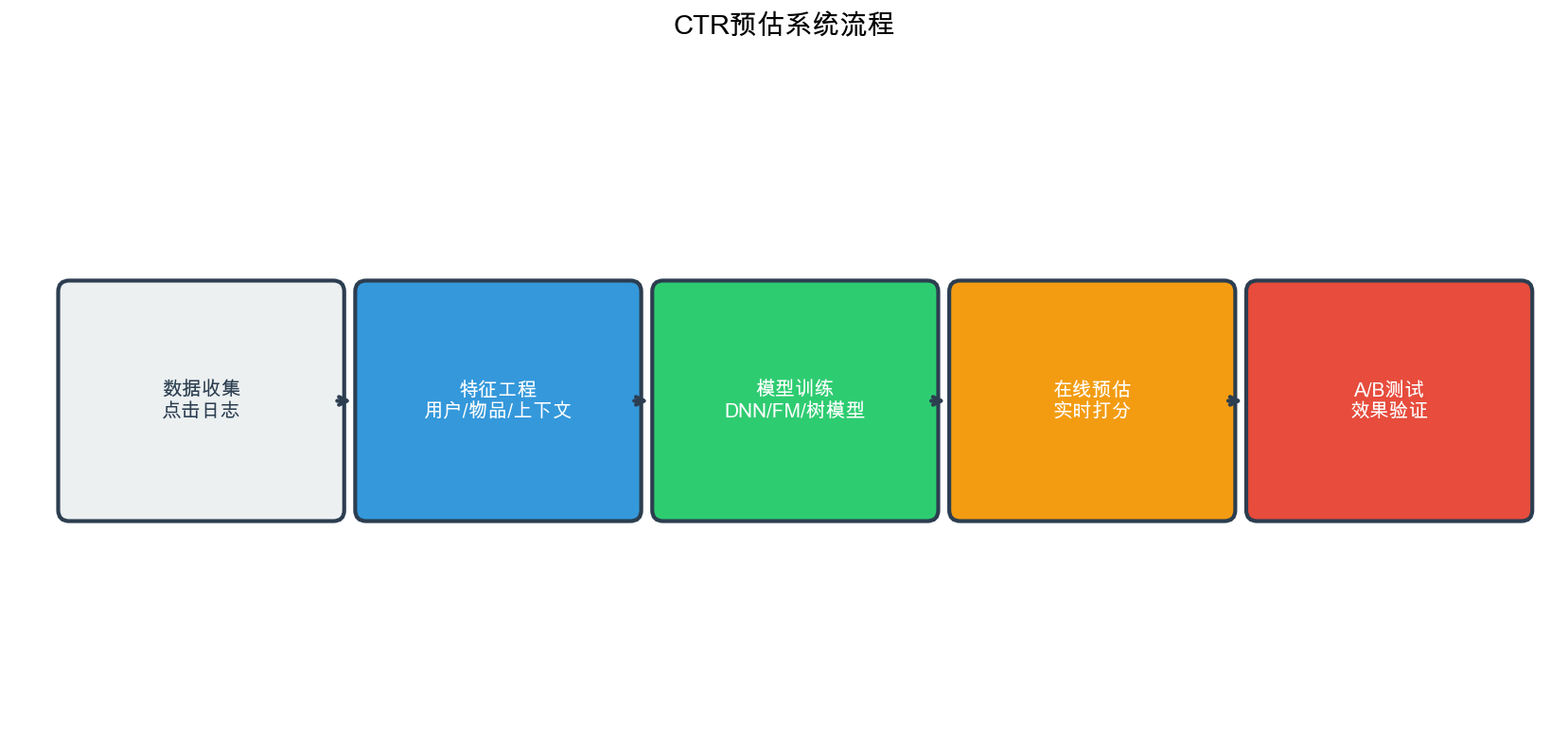
在推荐系统的排序阶段, CTR( Click-Through
Rate,点击率)预估是最核心的任务之一。无论是电商平台的商品推荐、信息流的内容推荐,还是广告系统的广告投放,都需要准确预测用户点击某个物品的概率。
CTR 预估的准确性直接影响用户体验和平台收益:提升 1%的 CTR
可能带来数百万的收入增长。
CTR
预估问题看似简单——给定用户特征、物品特征和上下文特征,预测用户点击的概率——但实际上充满了挑战。特征维度极高(百万到千万级)、特征极度稀疏(
99%以上都是
0)、特征交互复杂(二阶、三阶甚至更高阶的交互都很重要)、数据分布不平衡(点击样本通常只占
1-5%)。从 2010 年 Factorization Machines 提出开始, CTR
预估模型经历了从线性模型到因子分解机、再到深度学习模型的演进历程。
DeepFM 、 xDeepFM 、 DCN 、 AutoInt 、 FiBiNet 等模型不断刷新着 CTR
预估的 SOTA( State-of-the-Art)性能。
本文系统梳理 CTR
预估的核心问题、主流模型和实现细节。我们将从问题定义开始,理解 CTR
预估的本质;然后深入 Logistic Regression 、 FM 、 FFM
等经典模型;接着重点讲解 DeepFM 、 xDeepFM 、 DCN 、 AutoInt 、 FiBiNet
等深度学习模型;最后通过 10+个完整的代码实现和 10+个 Q&A
解答常见问题。无论你是 CTR 预估的新手,还是想系统掌握深度学习 CTR
模型,这篇文章都能帮你建立完整的知识体系。
CTR 预估问题定义
什么是 CTR 预估
CTR( Click-Through Rate)定义为:在给定展示(
impression)的情况下,用户点击( click)的概率。数学上可以表示为:
点 击 数 展 示 数
其中
CTR 预估的应用场景
CTR 预估在推荐系统的多个环节都有应用:
排序阶段( Ranking) : -
在召回阶段得到候选物品后,需要根据 CTR 对物品进行排序 - 通常与
CVR(转化率)、 GMV(成交总额)等指标结合,形成综合排序分数
广告投放( Advertising) : - eCPM( effective Cost
Per Mille)= CTR × CPC( Cost Per Click)× 1000 - 广告平台需要预估 CTR
来优化广告投放和竞价策略
内容推荐( Content Recommendation) : -
信息流推荐(如今日头条、微博)需要预估用户对内容的点击概率 -
视频推荐(如 YouTube 、抖音)需要预估用户对视频的点击概率
CTR 预估的挑战
CTR 预估面临以下主要挑战:
特征维度极高 : - 用户 ID 、物品 ID 等类别特征经过
one-hot 编码后,特征维度可达百万到千万级 - 例如,如果有 1000
万用户,仅用户 ID 特征就需要 1000 万维
特征极度稀疏 : -
每个样本只有极少数特征非零(通常只有几十到几百个) - 稀疏度可达
99.9%以上,即 99.9%的特征值都是 0
特征交互复杂 : -
一阶特征(如用户年龄、物品类别)很重要 -
二阶特征交互(如"年轻用户×电子产品")也很重要 -
高阶特征交互(如"年轻用户×电子产品×工作日×晚上")可能更重要
数据分布不平衡 : - 点击样本通常只占
1-5%,未点击样本占 95-99% - 需要合适的采样策略和损失函数设计
冷启动问题 : - 新用户、新物品缺乏历史数据 -
需要利用内容特征、相似用户/物品等辅助信息
CTR 预估的评价指标
CTR 预估常用的评价指标包括:
AUC( Area Under ROC Curve) : -
最常用的指标,衡量模型区分正负样本的能力 - AUC = 0.5 表示随机猜测, AUC
= 1.0 表示完美分类 - 通常 AUC > 0.75 认为模型可用, AUC > 0.80
认为模型较好
LogLoss(对数损失) : - 直接优化 LogLoss 通常能提升
AUC - LogLoss =准确率(
Accuracy) : - 在 CTR 预估中不太常用,因为正负样本不平衡
F1-Score : - 在需要平衡精确率和召回率时使用
Logistic Regression:
CTR 预估的基线模型
模型定义
Logistic Regression( LR)是 CTR 预估最基础的模型,它将 CTR
预估问题转化为二分类问题:
其中: -
为什么使用 Sigmoid 函数
Sigmoid 函数具有以下优点: 1.
输出范围 :将任意实数映射到[0,1]区间,符合概率的定义 2.
可导性 :处处可导,便于梯度下降优化 3.
概率解释 :输出可以解释为点击概率
LR 的优缺点
优点 : - 模型简单,训练和预测速度快 -
可解释性强,权重
缺点 : - 只能捕捉线性关系,无法捕捉特征交互 -
需要大量人工特征工程(如"用户年龄×物品类别") -
对于复杂的非线性模式,表达能力有限
LR 的实现
1
2
3
4
5
6
7
8
9
10
11
12
13
14
15
16
17
18
19
20
21
22
23
24
25
26
27
28
29
30
31
32
33
34
35
36
37
38
39
40
import numpy as npimport torchimport torch.nn as nnfrom torch.optim import Adamclass LogisticRegression (nn.Module): """Logistic Regression 模型""" def __init__ (self, feature_dim ): super (LogisticRegression, self).__init__() self.linear = nn.Linear(feature_dim, 1 ) def forward (self, x ): """ Args: x: [batch_size, feature_dim] 特征矩阵 Returns: logits: [batch_size, 1] 未经过 sigmoid 的分数 """ logits = self.linear(x) return logits def predict_proba (self, x ): """预测点击概率""" logits = self.forward(x) return torch.sigmoid(logits) model = LogisticRegression(feature_dim=10000 ) criterion = nn.BCEWithLogitsLoss() optimizer = Adam(model.parameters(), lr=0.001 ) for epoch in range (10 ): for batch_x, batch_y in train_loader: optimizer.zero_grad() logits = model(batch_x) loss = criterion(logits, batch_y.float ()) loss.backward() optimizer.step()
特征工程的重要性
在 LR 模型中,特征工程至关重要。常见的特征工程包括:
类别特征交叉 : - 用户 ID × 物品 ID - 用户年龄 ×
物品类别 - 用户性别 × 物品品牌
统计特征 : - 用户历史点击率 - 物品历史点击率 -
用户-物品历史交互次数
时间特征 : - 小时、星期、月份 -
是否工作日、是否节假日
Factorization
Machines( FM):捕捉二阶特征交互
FM 的提出背景
2010 年, Steffen Rendle 提出了 Factorization Machines( FM),解决了
LR 无法捕捉特征交互的问题。 FM
的基本思路:用向量内积来建模特征交互,而不是用独立的权重参数 。
FM 模型定义
FM 模型的预测公式为:
其中: -
FM 的核心创新
FM
的核心创新在于用隐向量的内积 来建模特征交互,而不是为每个特征对
参数共享 : - 传统方法需要
泛化能力 : - 即使特征对
FM 的计算优化
直接计算二阶项需要
这个变换将双重求和转化为单重求和,大大提高了计算效率。
FM 的实现
1
2
3
4
5
6
7
8
9
10
11
12
13
14
15
16
17
18
19
20
21
22
23
24
25
26
27
28
29
30
31
32
33
34
35
36
37
38
39
40
41
42
43
44
45
46
47
48
49
50
51
52
53
54
55
56
57
58
59
60
import torchimport torch.nn as nnclass FactorizationMachine (nn.Module): """Factorization Machine 模型""" def __init__ (self, feature_dim, embedding_dim=10 ): super (FactorizationMachine, self).__init__() self.feature_dim = feature_dim self.embedding_dim = embedding_dim self.linear = nn.Linear(feature_dim, 1 ) self.embeddings = nn.Embedding(feature_dim, embedding_dim) nn.init.xavier_uniform_(self.embeddings.weight) def forward (self, x ): """ Args: x: [batch_size, feature_dim] 特征矩阵(稀疏,大部分为 0) Returns: logits: [batch_size, 1] 预测分数 """ batch_size = x.size(0 ) linear_part = self.linear(x) nonzero_indices = x.nonzero(as_tuple=False ) nonzero_values = x[nonzero_indices[:, 0 ], nonzero_indices[:, 1 ]] fm_part = torch.zeros(batch_size, 1 , device=x.device) for i in range (batch_size): sample_indices = nonzero_indices[nonzero_indices[:, 0 ] == i, 1 ] sample_values = nonzero_values[nonzero_indices[:, 0 ] == i] if len (sample_indices) > 0 : embeds = self.embeddings(sample_indices) weighted_embeds = embeds * sample_values.unsqueeze(1 ) sum_square = torch.sum (weighted_embeds, dim=0 ) ** 2 square_sum = torch.sum (weighted_embeds ** 2 , dim=0 ) fm_part[i] = 0.5 * torch.sum (sum_square - square_sum) return linear_part + fm_part def predict_proba (self, x ): """预测点击概率""" logits = self.forward(x) return torch.sigmoid(logits)
在实际应用中,输入特征通常是稀疏的( one-hot 编码),可以优化 FM
的实现:
1
2
3
4
5
6
7
8
9
10
11
12
13
14
15
16
17
18
19
20
21
22
23
24
25
26
27
28
29
30
31
32
33
34
35
36
37
38
39
40
41
42
43
class SparseFactorizationMachine (nn.Module): """支持稀疏输入的 FM 模型""" def __init__ (self, feature_dim, embedding_dim=10 ): super (SparseFactorizationMachine, self).__init__() self.feature_dim = feature_dim self.embedding_dim = embedding_dim self.w0 = nn.Parameter(torch.zeros(1 )) self.w = nn.Embedding(feature_dim, 1 ) self.v = nn.Embedding(feature_dim, embedding_dim) nn.init.xavier_uniform_(self.w.weight) nn.init.xavier_uniform_(self.v.weight) def forward (self, feature_ids, feature_values ): """ Args: feature_ids: [batch_size, num_features] 特征 ID(稀疏表示) feature_values: [batch_size, num_features] 特征值(通常是 1.0) Returns: logits: [batch_size, 1] """ batch_size = feature_ids.size(0 ) w_embeds = self.w(feature_ids) linear_part = self.w0 + torch.sum (w_embeds.squeeze(-1 ) * feature_values, dim=1 , keepdim=True ) v_embeds = self.v(feature_ids) weighted_v = v_embeds * feature_values.unsqueeze(-1 ) sum_square = torch.sum (weighted_v, dim=1 ) ** 2 square_sum = torch.sum (weighted_v ** 2 , dim=1 ) fm_part = 0.5 * torch.sum (sum_square - square_sum, dim=1 , keepdim=True ) return linear_part + fm_part
Field-aware
Factorization Machines( FFM):考虑特征域
FFM 的提出
2016 年, Yu-Chin Juan 等人提出了 Field-aware Factorization
Machines( FFM),在 FM
的基础上引入了Field(域) 的概念。 FFM
认为:不同域(
Field)之间的特征交互应该使用不同的隐向量 。
Field 的概念
在 CTR 预估中,特征通常可以分为多个域( Field): -
用户域 :用户 ID 、用户年龄、用户性别等 -
物品域 :物品 ID 、物品类别、物品价格等 -
上下文域 :时间、地点、设备等
例如,在电商推荐中: - Field 1:用户 ID - Field 2:物品 ID - Field
3:用户年龄 - Field 4:物品类别 - Field 5:时间
FFM 模型定义
FFM 模型的预测公式为:
其中: -
FFM vs FM
FM : - 每个特征只有一个隐向量FFM : -
每个特征对每个域都有一个隐向量
FFM 的实现
1
2
3
4
5
6
7
8
9
10
11
12
13
14
15
16
17
18
19
20
21
22
23
24
25
26
27
28
29
30
31
32
33
34
35
36
37
38
39
40
41
42
43
44
45
46
47
48
49
50
51
52
53
54
55
56
57
58
59
60
61
62
63
64
65
66
67
68
69
70
71
72
73
74
75
class FieldAwareFactorizationMachine (nn.Module): """Field-aware Factorization Machine 模型""" def __init__ (self, feature_dim, num_fields, embedding_dim=10 ): super (FieldAwareFactorizationMachine, self).__init__() self.feature_dim = feature_dim self.num_fields = num_fields self.embedding_dim = embedding_dim self.w0 = nn.Parameter(torch.zeros(1 )) self.w = nn.Embedding(feature_dim, 1 ) self.v = nn.ModuleList([ nn.Embedding(feature_dim, embedding_dim) for _ in range (num_fields) ]) nn.init.xavier_uniform_(self.w.weight) for embed in self.v: nn.init.xavier_uniform_(embed.weight) def forward (self, feature_ids, feature_values, field_ids ): """ Args: feature_ids: [batch_size, num_features] 特征 ID feature_values: [batch_size, num_features] 特征值 field_ids: [batch_size, num_features] 特征所属的域 ID Returns: logits: [batch_size, 1] """ batch_size = feature_ids.size(0 ) w_embeds = self.w(feature_ids) linear_part = self.w0 + torch.sum (w_embeds.squeeze(-1 ) * feature_values, dim=1 , keepdim=True ) fm_part = torch.zeros(batch_size, 1 , device=feature_ids.device) for i in range (batch_size): sample_feature_ids = feature_ids[i] sample_feature_values = feature_values[i] sample_field_ids = field_ids[i] nonzero_mask = sample_feature_values > 0 nonzero_feature_ids = sample_feature_ids[nonzero_mask] nonzero_feature_values = sample_feature_values[nonzero_mask] nonzero_field_ids = sample_field_ids[nonzero_mask] num_nonzero = len (nonzero_feature_ids) for p in range (num_nonzero): for q in range (p + 1 , num_nonzero): feature_p_id = nonzero_feature_ids[p] feature_q_id = nonzero_feature_ids[q] field_p_id = nonzero_field_ids[p] field_q_id = nonzero_field_ids[q] value_p = nonzero_feature_values[p] value_q = nonzero_feature_values[q] v_p_fq = self.v[field_q_id](feature_p_id) v_q_fp = self.v[field_p_id](feature_q_id) interaction = torch.dot(v_p_fq, v_q_fp) * value_p * value_q fm_part[i] += interaction return linear_part + fm_part
FFM 的优缺点
优点 : - 考虑了特征域的信息,表达能力更强 - 在
Criteo 、 Avazu 等数据集上表现优于 FM
缺点 : - 参数量大(
DeepFM:结合深度学习和 FM
DeepFM 的提出
2017 年,华为诺亚方舟实验室提出了 DeepFM 模型,将Wide &
Deep
架构 和FM 结合,同时捕捉低阶和高阶特征交互。
DeepFM 的架构
DeepFM 由两部分组成:
FM 部分(低阶特征交互) : - 捕捉一阶和二阶特征交互 -
与传统的 FM 相同
Deep 部分(高阶特征交互) : - 多层全连接神经网络 -
自动学习高阶特征交互
两部分共享 Embedding 层,端到端训练:
其中: -
DeepFM 的架构图
1
2
3
4
5
6
7
8
9
10
11
12
输入特征 (稀疏) ↓ Embedding 层 (共享) ↓ ├──────────────┐ ↓ ↓ FM 部分 Deep 部分 (二阶交互) (多层 DNN) ↓ ↓ └──────┬───────┘ ↓ 输出层 (sigmoid)
DeepFM 的实现
1
2
3
4
5
6
7
8
9
10
11
12
13
14
15
16
17
18
19
20
21
22
23
24
25
26
27
28
29
30
31
32
33
34
35
36
37
38
39
40
41
42
43
44
45
46
47
48
49
50
51
52
53
54
55
56
57
58
59
60
61
62
63
64
class DeepFM (nn.Module): """DeepFM 模型""" def __init__ (self, feature_dim, embedding_dim=10 , hidden_dims=[128 , 64 ], dropout=0.5 ): super (DeepFM, self).__init__() self.feature_dim = feature_dim self.embedding_dim = embedding_dim self.w0 = nn.Parameter(torch.zeros(1 )) self.w = nn.Embedding(feature_dim, 1 ) self.embeddings = nn.Embedding(feature_dim, embedding_dim) deep_layers = [] input_dim = feature_dim * embedding_dim for hidden_dim in hidden_dims: deep_layers.append(nn.Linear(input_dim, hidden_dim)) deep_layers.append(nn.BatchNorm1d(hidden_dim)) deep_layers.append(nn.ReLU()) deep_layers.append(nn.Dropout(dropout)) input_dim = hidden_dim deep_layers.append(nn.Linear(input_dim, 1 )) self.deep = nn.Sequential(*deep_layers) nn.init.xavier_uniform_(self.w.weight) nn.init.xavier_uniform_(self.embeddings.weight) def forward (self, feature_ids, feature_values ): """ Args: feature_ids: [batch_size, num_features] 特征 ID feature_values: [batch_size, num_features] 特征值 Returns: logits: [batch_size, 1] """ batch_size = feature_ids.size(0 ) w_embeds = self.w(feature_ids) linear_part = self.w0 + torch.sum (w_embeds.squeeze(-1 ) * feature_values, dim=1 , keepdim=True ) v_embeds = self.embeddings(feature_ids) weighted_v = v_embeds * feature_values.unsqueeze(-1 ) sum_square = torch.sum (weighted_v, dim=1 ) ** 2 square_sum = torch.sum (weighted_v ** 2 , dim=1 ) fm_part = 0.5 * torch.sum (sum_square - square_sum, dim=1 , keepdim=True ) deep_input = weighted_v.view(batch_size, -1 ) deep_part = self.deep(deep_input) return linear_part + fm_part + deep_part def predict_proba (self, feature_ids, feature_values ): """预测点击概率""" logits = self.forward(feature_ids, feature_values) return torch.sigmoid(logits)
DeepFM 的优势
结合低阶和高阶交互 : - FM 部分捕捉一阶和二阶交互 -
Deep 部分捕捉高阶交互 - 两者互补,提升模型表达能力
共享 Embedding : - FM 和 Deep 共享 Embedding
层,减少参数量 - 端到端训练,优化更充分
无需特征工程 : - Deep
部分自动学习特征交互,减少人工特征工程
DeepFM vs Wide & Deep
Wide & Deep : - Wide 部分需要人工设计交叉特征 -
Deep 部分学习高阶交互
DeepFM : - FM 部分自动学习二阶交互(无需人工设计) -
Deep 部分学习高阶交互 - 比 Wide & Deep 更自动化
xDeepFM:显式高阶特征交互
xDeepFM 的提出
2018 年,中科大和微软提出了 xDeepFM( eXtreme Deep Factorization
Machine),在 DeepFM 的基础上引入了CIN( Compressed Interaction
Network) ,显式地建模高阶特征交互。
CIN 的核心思想
CIN
的基本思路:显式地建模特征交互,而不是依赖深度神经网络的隐式学习 。
CIN 通过以下方式工作: 1. 第
CIN 的数学定义
设
其中: -
xDeepFM 的架构
xDeepFM = Linear 部分 + CIN 部分 +
DNN 部分
Linear 部分 :一阶特征权重CIN 部分 :显式高阶特征交互DNN 部分 :隐式高阶特征交互
xDeepFM 的实现
1
2
3
4
5
6
7
8
9
10
11
12
13
14
15
16
17
18
19
20
21
22
23
24
25
26
27
28
29
30
31
32
33
34
35
36
37
38
39
40
41
42
43
44
45
46
47
48
49
50
51
52
53
54
55
56
57
58
59
60
61
62
63
64
65
66
67
68
69
70
71
72
73
74
75
76
77
78
79
80
81
82
83
84
85
86
87
88
89
90
91
92
93
94
95
96
97
98
99
100
101
102
103
104
105
106
107
108
109
110
111
112
113
114
115
116
117
118
119
120
121
122
123
124
125
126
127
128
129
130
131
132
133
134
135
136
137
138
139
140
141
142
143
144
145
146
147
148
149
150
151
class CIN (nn.Module): """Compressed Interaction Network""" def __init__ (self, input_dim, cin_layer_sizes=[100 , 100 ] ): super (CIN, self).__init__() self.input_dim = input_dim self.cin_layer_sizes = cin_layer_sizes self.cin_layers = nn.ModuleList() prev_size = input_dim for size in cin_layer_sizes: layer = nn.Conv1d( in_channels=prev_size, out_channels=size, kernel_size=1 , stride=1 , padding=0 ) self.cin_layers.append(layer) prev_size = size def forward (self, x0 ): """ Args: x0: [batch_size, num_fields, embedding_dim] 原始 embedding Returns: output: [batch_size, sum(cin_layer_sizes)] CIN 的输出 """ batch_size = x0.size(0 ) num_fields = x0.size(1 ) embedding_dim = x0.size(2 ) x_list = [x0] for cin_layer in self.cin_layers: x_k_minus_1 = x_list[-1 ] x_k_minus_1_expanded = x_k_minus_1.unsqueeze(2 ) x0_expanded = x0.unsqueeze(1 ) z_k = x_k_minus_1_expanded * x0_expanded z_k = z_k.view(batch_size, -1 , embedding_dim) x_k = cin_layer(z_k) x_list.append(x_k) cin_outputs = [] for x in x_list[1 :]: cin_outputs.append(torch.sum (x, dim=2 )) output = torch.cat(cin_outputs, dim=1 ) return output class xDeepFM (nn.Module): """xDeepFM 模型""" def __init__ (self, feature_dim, num_fields, embedding_dim=10 , cin_layer_sizes=[100 , 100 ], dnn_hidden_dims=[128 , 64 ], dropout=0.5 ): super (xDeepFM, self).__init__() self.feature_dim = feature_dim self.num_fields = num_fields self.embedding_dim = embedding_dim self.w0 = nn.Parameter(torch.zeros(1 )) self.w = nn.Embedding(feature_dim, 1 ) self.embeddings = nn.Embedding(feature_dim, embedding_dim) self.cin = CIN(embedding_dim, cin_layer_sizes) cin_output_dim = sum (cin_layer_sizes) dnn_input_dim = num_fields * embedding_dim dnn_layers = [] for hidden_dim in dnn_hidden_dims: dnn_layers.append(nn.Linear(dnn_input_dim, hidden_dim)) dnn_layers.append(nn.BatchNorm1d(hidden_dim)) dnn_layers.append(nn.ReLU()) dnn_layers.append(nn.Dropout(dropout)) dnn_input_dim = hidden_dim dnn_layers.append(nn.Linear(dnn_input_dim, 1 )) self.dnn = nn.Sequential(*dnn_layers) nn.init.xavier_uniform_(self.w.weight) nn.init.xavier_uniform_(self.embeddings.weight) def forward (self, feature_ids, feature_values, field_ids ): """ Args: feature_ids: [batch_size, num_features] 特征 ID feature_values: [batch_size, num_features] 特征值 field_ids: [batch_size, num_features] 特征所属的域 ID Returns: logits: [batch_size, 1] """ batch_size = feature_ids.size(0 ) w_embeds = self.w(feature_ids) linear_part = self.w0 + torch.sum (w_embeds.squeeze(-1 ) * feature_values, dim=1 , keepdim=True ) v_embeds = self.embeddings(feature_ids) weighted_v = v_embeds * feature_values.unsqueeze(-1 ) field_embeds = [] for field_id in range (self.num_fields): field_mask = (field_ids == field_id) if field_mask.any (): field_embed = weighted_v[:, field_mask, :].sum (dim=1 ) else : field_embed = torch.zeros(batch_size, self.embedding_dim, device=feature_ids.device) field_embeds.append(field_embed) field_embeds = torch.stack(field_embeds, dim=1 ) cin_output = self.cin(field_embeds) cin_part = torch.sum (cin_output, dim=1 , keepdim=True ) dnn_input = field_embeds.view(batch_size, -1 ) dnn_part = self.dnn(dnn_input) return linear_part + cin_part + dnn_part
xDeepFM 的优势
显式高阶交互 : - CIN
显式地建模高阶特征交互,可解释性更强 - 比 DNN 的隐式学习更可控
结合显式和隐式 : - CIN 捕捉显式交互 - DNN
捕捉隐式交互 - 两者互补
Deep & Cross Network(
DCN):交叉网络
DCN 的提出
2017 年, Google 提出了 Deep & Cross Network(
DCN),引入了Cross Network 来显式建模特征交互。
Cross Network 的核心思想
Cross Network 通过以下方式工作: 1. 每一层都是原始输入和上一层的交叉
2. 逐层构建高阶交互 3. 参数量少,计算高效
Cross Network 的数学定义
设
其中: -
DCN 的架构
DCN = Cross Network + Deep
Network
Cross Network :显式特征交互Deep Network :隐式特征交互
DCN 的实现
1
2
3
4
5
6
7
8
9
10
11
12
13
14
15
16
17
18
19
20
21
22
23
24
25
26
27
28
29
30
31
32
33
34
35
36
37
38
39
40
41
42
43
44
45
46
47
48
49
50
51
52
53
54
55
56
57
58
59
60
61
62
63
64
65
66
67
68
69
70
71
72
73
74
75
76
77
78
79
80
81
82
83
84
85
86
87
88
89
90
91
92
93
94
95
96
97
98
99
100
101
102
103
104
105
106
107
108
109
110
111
112
113
114
115
116
117
118
119
120
121
122
class CrossNetwork (nn.Module): """Cross Network""" def __init__ (self, input_dim, num_layers=3 ): super (CrossNetwork, self).__init__() self.input_dim = input_dim self.num_layers = num_layers self.cross_weights = nn.ModuleList([ nn.Linear(input_dim, 1 , bias=False ) for _ in range (num_layers) ]) self.cross_bias = nn.ParameterList([ nn.Parameter(torch.zeros(input_dim)) for _ in range (num_layers) ]) def forward (self, x0 ): """ Args: x0: [batch_size, input_dim] 原始输入 Returns: x_l: [batch_size, input_dim] Cross Network 的输出 """ x_l = x0 for i in range (self.num_layers): xlw = self.cross_weights[i](x_l) xl_next = x0 * xlw + self.cross_bias[i] + x_l x_l = xl_next return x_l class DeepCrossNetwork (nn.Module): """Deep & Cross Network""" def __init__ (self, feature_dim, embedding_dim=10 , num_fields=None , cross_num_layers=3 , dnn_hidden_dims=[128 , 64 ], dropout=0.5 ): super (DeepCrossNetwork, self).__init__() self.feature_dim = feature_dim self.embedding_dim = embedding_dim if num_fields is None : num_fields = feature_dim self.embeddings = nn.Embedding(feature_dim, embedding_dim) cross_input_dim = num_fields * embedding_dim self.cross_net = CrossNetwork(cross_input_dim, cross_num_layers) dnn_layers = [] dnn_input_dim = cross_input_dim for hidden_dim in dnn_hidden_dims: dnn_layers.append(nn.Linear(dnn_input_dim, hidden_dim)) dnn_layers.append(nn.BatchNorm1d(hidden_dim)) dnn_layers.append(nn.ReLU()) dnn_layers.append(nn.Dropout(dropout)) dnn_input_dim = hidden_dim dnn_layers.append(nn.Linear(dnn_input_dim, 1 )) self.dnn = nn.Sequential(*dnn_layers) self.final_linear = nn.Linear(cross_input_dim + dnn_hidden_dims[-1 ], 1 ) nn.init.xavier_uniform_(self.embeddings.weight) def forward (self, feature_ids, feature_values, field_ids=None ): """ Args: feature_ids: [batch_size, num_features] 特征 ID feature_values: [batch_size, num_features] 特征值 field_ids: [batch_size, num_features] 特征所属的域 ID(可选) Returns: logits: [batch_size, 1] """ batch_size = feature_ids.size(0 ) v_embeds = self.embeddings(feature_ids) weighted_v = v_embeds * feature_values.unsqueeze(-1 ) if field_ids is None : cross_input = weighted_v.view(batch_size, -1 ) else : num_fields = field_ids.max ().item() + 1 field_embeds = [] for field_id in range (num_fields): field_mask = (field_ids == field_id) if field_mask.any (): field_embed = weighted_v[:, field_mask, :].sum (dim=1 ) else : field_embed = torch.zeros(batch_size, self.embedding_dim, device=feature_ids.device) field_embeds.append(field_embed) cross_input = torch.stack(field_embeds, dim=1 ).view(batch_size, -1 ) cross_output = self.cross_net(cross_input) dnn_output = self.dnn(cross_input) concat_output = torch.cat([cross_output, dnn_output], dim=1 ) logits = self.final_linear(concat_output) return logits
DCN 的优势
高效的显式交互 : - Cross Network
参数量少(每层只有
结合显式和隐式 : - Cross Network 捕捉显式交互 - Deep
Network 捕捉隐式交互
AutoInt:基于 Attention
的特征交互
AutoInt 的提出
2019 年,北大和微软提出了 AutoInt( Automatic Feature Interaction
Learning),使用Multi-head
Self-Attention 来自动学习特征交互。
Attention 机制在 CTR
预估中的应用
Attention
机制的基本思路:学习特征之间的重要性权重,自动发现重要的特征交互 。
对于特征
其中: -
AutoInt 的架构
AutoInt = Embedding 层 + 多个 Interacting
层 + 输出层
每个 Interacting 层包含: 1. Multi-head Self-Attention 2. Residual
Connection 3. Feed-Forward Network
AutoInt 的实现
1
2
3
4
5
6
7
8
9
10
11
12
13
14
15
16
17
18
19
20
21
22
23
24
25
26
27
28
29
30
31
32
33
34
35
36
37
38
39
40
41
42
43
44
45
46
47
48
49
50
51
52
53
54
55
56
57
58
59
60
61
62
63
64
65
66
67
68
69
70
71
72
73
74
75
76
77
78
79
80
81
82
83
84
85
86
87
88
89
90
91
92
93
94
95
96
97
98
99
100
101
102
103
104
105
106
107
108
109
110
111
112
113
114
115
116
117
118
119
120
121
122
123
124
125
126
127
128
129
130
131
132
133
134
135
136
137
138
139
140
141
142
143
144
145
146
147
148
149
150
151
152
class MultiHeadSelfAttention (nn.Module): """Multi-head Self-Attention""" def __init__ (self, embedding_dim, num_heads=4 ): super (MultiHeadSelfAttention, self).__init__() assert embedding_dim % num_heads == 0 self.embedding_dim = embedding_dim self.num_heads = num_heads self.head_dim = embedding_dim // num_heads self.W_q = nn.Linear(embedding_dim, embedding_dim) self.W_k = nn.Linear(embedding_dim, embedding_dim) self.W_v = nn.Linear(embedding_dim, embedding_dim) self.W_o = nn.Linear(embedding_dim, embedding_dim) def forward (self, x ): """ Args: x: [batch_size, num_fields, embedding_dim] Returns: output: [batch_size, num_fields, embedding_dim] """ batch_size, num_fields, embedding_dim = x.size() Q = self.W_q(x) K = self.W_k(x) V = self.W_v(x) Q = Q.view(batch_size, num_fields, self.num_heads, self.head_dim).transpose(1 , 2 ) K = K.view(batch_size, num_fields, self.num_heads, self.head_dim).transpose(1 , 2 ) V = V.view(batch_size, num_fields, self.num_heads, self.head_dim).transpose(1 , 2 ) scores = torch.matmul(Q, K.transpose(-2 , -1 )) / np.sqrt(self.head_dim) attn_weights = torch.softmax(scores, dim=-1 ) attn_output = torch.matmul(attn_weights, V) attn_output = attn_output.transpose(1 , 2 ).contiguous().view( batch_size, num_fields, embedding_dim ) output = self.W_o(attn_output) return output class InteractingLayer (nn.Module): """AutoInt 的 Interacting 层""" def __init__ (self, embedding_dim, num_heads=4 , dropout=0.1 ): super (InteractingLayer, self).__init__() self.attention = MultiHeadSelfAttention(embedding_dim, num_heads) self.feed_forward = nn.Sequential( nn.Linear(embedding_dim, embedding_dim * 4 ), nn.ReLU(), nn.Dropout(dropout), nn.Linear(embedding_dim * 4 , embedding_dim), nn.Dropout(dropout) ) self.norm1 = nn.LayerNorm(embedding_dim) self.norm2 = nn.LayerNorm(embedding_dim) def forward (self, x ): """ Args: x: [batch_size, num_fields, embedding_dim] Returns: output: [batch_size, num_fields, embedding_dim] """ attn_output = self.attention(x) x = self.norm1(x + attn_output) ff_output = self.feed_forward(x) x = self.norm2(x + ff_output) return x class AutoInt (nn.Module): """AutoInt 模型""" def __init__ (self, feature_dim, num_fields, embedding_dim=10 , num_layers=3 , num_heads=4 , dropout=0.1 ): super (AutoInt, self).__init__() self.feature_dim = feature_dim self.num_fields = num_fields self.embedding_dim = embedding_dim self.embeddings = nn.Embedding(feature_dim, embedding_dim) self.interacting_layers = nn.ModuleList([ InteractingLayer(embedding_dim, num_heads, dropout) for _ in range (num_layers) ]) self.output_layer = nn.Linear(num_fields * embedding_dim, 1 ) nn.init.xavier_uniform_(self.embeddings.weight) def forward (self, feature_ids, feature_values, field_ids ): """ Args: feature_ids: [batch_size, num_features] 特征 ID feature_values: [batch_size, num_features] 特征值 field_ids: [batch_size, num_features] 特征所属的域 ID Returns: logits: [batch_size, 1] """ batch_size = feature_ids.size(0 ) v_embeds = self.embeddings(feature_ids) weighted_v = v_embeds * feature_values.unsqueeze(-1 ) field_embeds = [] for field_id in range (self.num_fields): field_mask = (field_ids == field_id) if field_mask.any (): field_embed = weighted_v[:, field_mask, :].sum (dim=1 ) else : field_embed = torch.zeros(batch_size, self.embedding_dim, device=feature_ids.device) field_embeds.append(field_embed) x = torch.stack(field_embeds, dim=1 ) for layer in self.interacting_layers: x = layer(x) x_flat = x.view(batch_size, -1 ) logits = self.output_layer(x_flat) return logits
AutoInt 的优势
自动学习特征交互 : - Attention
机制自动发现重要的特征交互 - 无需人工设计交叉特征
可解释性 : - Attention
权重可以可视化,解释哪些特征交互最重要
灵活性 : - 可以捕捉任意阶的特征交互 - Multi-head
机制捕捉不同类型的交互模式
FiBiNet:特征重要性网络
FiBiNet 的提出
2019 年,新浪微博提出了 FiBiNet( Feature Importance and Bilinear
feature Interaction Network),引入了SENet(
Squeeze-and-Excitation
Network) 来学习特征重要性,并使用Bilinear
Interaction 来建模特征交互。
SENet:学习特征重要性
SENet
的基本思路:为每个特征学习一个重要性权重,动态调整特征的贡献 。
SENet 包含两个步骤: 1. Squeeze :对每个特征的
embedding 进行全局平均池化 2.
Excitation :通过两层全连接网络学习重要性权重
Bilinear
Interaction:建模特征交互
Bilinear Interaction 使用双线性函数来建模特征交互:
其中
FiBiNet 提出了三种 Bilinear Interaction: 1. Field-All
Type :所有 field 共享一个权重矩阵 2. Field-Each
Type :每个 field 有自己的权重矩阵 3. Field-Interaction
Type :每对 field 有一个权重矩阵
FiBiNet 的架构
FiBiNet = SENet 层 + Bilinear Interaction
层 + DNN 层
FiBiNet 的实现
1
2
3
4
5
6
7
8
9
10
11
12
13
14
15
16
17
18
19
20
21
22
23
24
25
26
27
28
29
30
31
32
33
34
35
36
37
38
39
40
41
42
43
44
45
46
47
48
49
50
51
52
53
54
55
56
57
58
59
60
61
62
63
64
65
66
67
68
69
70
71
72
73
74
75
76
77
78
79
80
81
82
83
84
85
86
87
88
89
90
91
92
93
94
95
96
97
98
99
100
101
102
103
104
105
106
107
108
109
110
111
112
113
114
115
116
117
118
119
120
121
122
123
124
125
126
127
128
129
130
131
132
133
134
135
136
137
138
139
140
141
142
143
144
145
146
147
148
149
150
151
152
153
154
155
156
157
158
159
160
161
162
163
164
165
166
167
168
169
170
171
172
173
174
175
176
177
178
179
180
181
182
183
184
185
186
class SENet (nn.Module): """Squeeze-and-Excitation Network""" def __init__ (self, num_fields, reduction_ratio=3 ): super (SENet, self).__init__() self.num_fields = num_fields reduced_dim = max (1 , num_fields // reduction_ratio) self.excitation = nn.Sequential( nn.Linear(num_fields, reduced_dim), nn.ReLU(), nn.Linear(reduced_dim, num_fields), nn.ReLU() ) def forward (self, x ): """ Args: x: [batch_size, num_fields, embedding_dim] Returns: output: [batch_size, num_fields, embedding_dim] """ z = torch.mean(x, dim=2 ) weights = self.excitation(z) weights = torch.sigmoid(weights).unsqueeze(-1 ) output = x * weights return output class BilinearInteraction (nn.Module): """Bilinear Interaction""" def __init__ (self, num_fields, embedding_dim, bilinear_type='field_interaction' ): super (BilinearInteraction, self).__init__() self.num_fields = num_fields self.embedding_dim = embedding_dim self.bilinear_type = bilinear_type if bilinear_type == 'field_all' : self.W = nn.Parameter(torch.randn(embedding_dim, embedding_dim)) elif bilinear_type == 'field_each' : self.W_list = nn.ParameterList([ nn.Parameter(torch.randn(embedding_dim, embedding_dim)) for _ in range (num_fields) ]) elif bilinear_type == 'field_interaction' : self.W_list = nn.ParameterList([ nn.Parameter(torch.randn(embedding_dim, embedding_dim)) for _ in range (num_fields * (num_fields - 1 ) // 2 ) ]) else : raise ValueError(f"Unknown bilinear_type: {bilinear_type} " ) def forward (self, x ): """ Args: x: [batch_size, num_fields, embedding_dim] Returns: output: [batch_size, num_fields * (num_fields - 1) // 2, embedding_dim] """ batch_size = x.size(0 ) num_fields = x.size(1 ) embedding_dim = x.size(2 ) p_list = [] idx = 0 for i in range (num_fields): for j in range (i + 1 , num_fields): v_i = x[:, i, :] v_j = x[:, j, :] if self.bilinear_type == 'field_all' : p_ij = torch.bmm( v_i.unsqueeze(1 ), self.W.unsqueeze(0 ).expand(batch_size, -1 , -1 ) ) p_ij = torch.bmm(p_ij, v_j.unsqueeze(-1 )) p_ij = p_ij.squeeze(-1 ) p_ij = (v_i * torch.matmul(v_j, self.W.t())).sum (dim=1 , keepdim=True ) elif self.bilinear_type == 'field_each' : p_ij = torch.sum (v_i * torch.matmul(v_j, self.W_list[i].t()), dim=1 , keepdim=True ) elif self.bilinear_type == 'field_interaction' : p_ij = torch.sum (v_i * torch.matmul(v_j, self.W_list[idx].t()), dim=1 , keepdim=True ) idx += 1 p_ij_vec = v_i * v_j p_list.append(p_ij_vec) output = torch.stack(p_list, dim=1 ) return output class FiBiNet (nn.Module): """FiBiNet 模型""" def __init__ (self, feature_dim, num_fields, embedding_dim=10 , reduction_ratio=3 , bilinear_type='field_interaction' , dnn_hidden_dims=[128 , 64 ], dropout=0.5 ): super (FiBiNet, self).__init__() self.feature_dim = feature_dim self.num_fields = num_fields self.embedding_dim = embedding_dim self.embeddings = nn.Embedding(feature_dim, embedding_dim) self.senet = SENet(num_fields, reduction_ratio) self.bilinear = BilinearInteraction(num_fields, embedding_dim, bilinear_type) num_pairs = num_fields * (num_fields - 1 ) // 2 bilinear_output_dim = num_pairs * embedding_dim dnn_layers = [] dnn_input_dim = bilinear_output_dim for hidden_dim in dnn_hidden_dims: dnn_layers.append(nn.Linear(dnn_input_dim, hidden_dim)) dnn_layers.append(nn.BatchNorm1d(hidden_dim)) dnn_layers.append(nn.ReLU()) dnn_layers.append(nn.Dropout(dropout)) dnn_input_dim = hidden_dim dnn_layers.append(nn.Linear(dnn_input_dim, 1 )) self.dnn = nn.Sequential(*dnn_layers) nn.init.xavier_uniform_(self.embeddings.weight) def forward (self, feature_ids, feature_values, field_ids ): """ Args: feature_ids: [batch_size, num_features] 特征 ID feature_values: [batch_size, num_features] 特征值 field_ids: [batch_size, num_features] 特征所属的域 ID Returns: logits: [batch_size, 1] """ batch_size = feature_ids.size(0 ) v_embeds = self.embeddings(feature_ids) weighted_v = v_embeds * feature_values.unsqueeze(-1 ) field_embeds = [] for field_id in range (self.num_fields): field_mask = (field_ids == field_id) if field_mask.any (): field_embed = weighted_v[:, field_mask, :].sum (dim=1 ) else : field_embed = torch.zeros(batch_size, self.embedding_dim, device=feature_ids.device) field_embeds.append(field_embed) x = torch.stack(field_embeds, dim=1 ) x_senet = self.senet(x) x_bilinear = self.bilinear(x_senet) x_bilinear_flat = x_bilinear.view(batch_size, -1 ) logits = self.dnn(x_bilinear_flat) return logits
FiBiNet 的优势
特征重要性学习 : - SENet 自动学习每个特征的重要性 -
动态调整特征的贡献,提升模型性能
灵活的特征交互 : - Bilinear Interaction 比内积更灵活
- 三种类型适应不同场景
完整代码实现:统一的训练框架
数据预处理
1
2
3
4
5
6
7
8
9
10
11
12
13
14
15
16
17
18
19
20
21
22
23
24
25
26
27
28
29
30
31
32
33
34
35
36
37
38
39
40
41
42
43
44
45
46
47
48
49
50
51
52
53
54
55
56
57
58
59
60
import pandas as pdimport numpy as npfrom sklearn.preprocessing import LabelEncoderfrom torch.utils.data import Dataset, DataLoaderclass CTRDataset (Dataset ): """CTR 预估数据集""" def __init__ (self, data_path, mode='train' ): self.data = pd.read_csv(data_path) self.mode = mode self.label_encoders = {} self.feature_columns = [] self.field_ids = [] self._preprocess() def _preprocess (self ): """预处理数据""" categorical_features = ['user_id' , 'item_id' , 'category' , 'brand' ] for col in categorical_features: if col in self.data.columns: le = LabelEncoder() self.data[col] = le.fit_transform(self.data[col].astype(str )) self.label_encoders[col] = le self.feature_columns.append(col) self.field_ids.append(len (self.field_ids)) def __len__ (self ): return len (self.data) def __getitem__ (self, idx ): row = self.data.iloc[idx] feature_ids = [] feature_values = [] field_ids_list = [] for i, col in enumerate (self.feature_columns): feature_ids.append(row[col]) feature_values.append(1.0 ) field_ids_list.append(self.field_ids[i]) feature_ids = torch.tensor(feature_ids, dtype=torch.long) feature_values = torch.tensor(feature_values, dtype=torch.float ) field_ids = torch.tensor(field_ids_list, dtype=torch.long) if self.mode == 'train' : label = torch.tensor(row['label' ], dtype=torch.float ) return feature_ids, feature_values, field_ids, label else : return feature_ids, feature_values, field_ids
训练脚本
1
2
3
4
5
6
7
8
9
10
11
12
13
14
15
16
17
18
19
20
21
22
23
24
25
26
27
28
29
30
31
32
33
34
35
36
37
38
39
40
41
42
43
44
45
46
47
48
49
50
51
52
53
54
55
56
57
58
59
60
61
62
63
64
65
66
67
68
69
70
71
72
73
74
75
76
77
78
import torchimport torch.nn as nnfrom torch.optim import Adamfrom torch.utils.data import DataLoaderfrom sklearn.metrics import roc_auc_score, log_lossimport numpy as npdef train_model (model, train_loader, val_loader, num_epochs=10 , lr=0.001 ): """训练 CTR 模型""" device = torch.device('cuda' if torch.cuda.is_available() else 'cpu' ) model = model.to(device) criterion = nn.BCEWithLogitsLoss() optimizer = Adam(model.parameters(), lr=lr) best_auc = 0.0 for epoch in range (num_epochs): model.train() train_loss = 0.0 train_preds = [] train_labels = [] for batch in train_loader: feature_ids, feature_values, field_ids, labels = batch feature_ids = feature_ids.to(device) feature_values = feature_values.to(device) field_ids = field_ids.to(device) labels = labels.to(device) optimizer.zero_grad() logits = model(feature_ids, feature_values, field_ids).squeeze() loss = criterion(logits, labels) loss.backward() optimizer.step() train_loss += loss.item() train_preds.extend(torch.sigmoid(logits).detach().cpu().numpy()) train_labels.extend(labels.cpu().numpy()) train_loss /= len (train_loader) train_auc = roc_auc_score(train_labels, train_preds) model.eval () val_loss = 0.0 val_preds = [] val_labels = [] with torch.no_grad(): for batch in val_loader: feature_ids, feature_values, field_ids, labels = batch feature_ids = feature_ids.to(device) feature_values = feature_values.to(device) field_ids = field_ids.to(device) labels = labels.to(device) logits = model(feature_ids, feature_values, field_ids).squeeze() loss = criterion(logits, labels) val_loss += loss.item() val_preds.extend(torch.sigmoid(logits).cpu().numpy()) val_labels.extend(labels.cpu().numpy()) val_loss /= len (val_loader) val_auc = roc_auc_score(val_labels, val_preds) print (f"Epoch {epoch+1 } /{num_epochs} " ) print (f"Train Loss: {train_loss:.4 f} , Train AUC: {train_auc:.4 f} " ) print (f"Val Loss: {val_loss:.4 f} , Val AUC: {val_auc:.4 f} " ) if val_auc > best_auc: best_auc = val_auc torch.save(model.state_dict(), 'best_model.pth' ) return model
Q&A:常见问题解答
Q1: 为什么 CTR 预估使用
AUC 而不是准确率?
A : CTR 预估中正负样本极度不平衡(点击样本通常只占
1-5%),如果使用准确率,模型可能简单地预测所有样本为负样本就能获得
95%的准确率,但这没有意义。 AUC
衡量的是模型区分正负样本的能力,不受类别不平衡影响,更适合 CTR
预估任务。
Q2: FM 为什么能处理稀疏特征?
A : FM
通过隐向量的内积来建模特征交互,即使某个特征对
Q3:
DeepFM 中 FM 部分和 Deep 部分为什么要共享 Embedding?
A : 共享 Embedding 有以下几个好处: 1.
减少参数量 :如果 FM 和 Deep 各自有独立的
Embedding,参数量会翻倍 2. 信息共享 : FM
部分学习到的低阶交互信息可以通过共享的 Embedding 传递给 Deep 部分 3.
端到端训练 :共享 Embedding
使得整个模型可以端到端训练,优化更充分
Q4: xDeepFM 的 CIN 和 DNN
有什么区别?
A : -
CIN :显式地建模特征交互,每一层的输出都是原始输入和上一层的交叉,可解释性更强
-
DNN :隐式地学习特征交互,通过多层非线性变换自动学习,表达能力更强但可解释性较差
- 两者互补: CIN 捕捉显式交互, DNN 捕捉隐式交互
A : AutoInt 的 Attention 机制借鉴了 Transformer 的
Multi-head Self-Attention,但有以下区别: 1. 应用场景 :
Transformer 主要用于序列建模, AutoInt 用于特征交互 2.
输入 : Transformer 的输入是序列, AutoInt
的输入是特征集合(无序) 3. 位置编码 : Transformer
需要位置编码, AutoInt 不需要(特征没有顺序)
Q6: FiBiNet 的 SENet
为什么能提升性能?
A : SENet
通过学习特征重要性权重,动态调整每个特征的贡献。对于不重要的特征,权重会较小,减少噪声;对于重要的特征,权重会较大,增强信号。这种自适应机制使得模型能够更好地关注重要的特征,提升性能。
Q7: 如何选择 CTR 预估模型?
A : 选择模型需要考虑以下因素: 1.
数据规模 :数据量大时可以选择更复杂的模型(如 xDeepFM 、
AutoInt) 2.
特征复杂度 :特征交互复杂时选择显式建模交互的模型(如
xDeepFM 、 DCN) 3.
计算资源 :计算资源有限时选择简单的模型(如 FM 、
DeepFM) 4. 可解释性要求 :需要可解释性时选择 FM 、
xDeepFM 等模型
Q8: CTR
预估中如何处理类别特征?
A : 类别特征通常通过以下方式处理: 1. One-hot
编码 :将类别特征转换为稀疏向量 2.
Embedding :将类别特征映射到低维稠密向量(最常用) 3.
Hash 编码 :对于高基数类别特征,使用 Hash
函数映射到固定维度
Q9: 如何解决 CTR
预估中的数据不平衡问题?
A : 可以采用以下方法: 1.
负采样 :对负样本进行采样,平衡正负样本比例 2.
Focal Loss :使用 Focal Loss,自动调整难易样本的权重 3.
AUC 优化 :直接优化 AUC 而不是 LogLoss 4.
集成学习 :使用多个模型集成,提升性能
Q10: CTR
预估模型的训练技巧有哪些?
A : 常用的训练技巧包括: 1.
学习率调度 :使用学习率衰减策略(如 ReduceLROnPlateau)
2. 正则化 :使用 L1/L2 正则化防止过拟合 3. Batch
Normalization :加速训练,提升稳定性 4.
Dropout :防止过拟合 5. 早停( Early
Stopping) :防止过拟合 6.
特征归一化 :对连续特征进行归一化
Q11: 如何评估 CTR
预估模型的效果?
A : 评估 CTR 预估模型通常使用以下指标: 1.
AUC :最常用的指标,衡量模型区分正负样本的能力 2.
LogLoss :直接优化 LogLoss 通常能提升 AUC 3.
线上 A/B 测试 :在真实环境中测试模型效果 4.
业务指标 : CTR 、 GMV 、用户停留时长等业务指标
Q12: CTR
预估模型如何部署到生产环境?
A : 部署 CTR 预估模型需要考虑: 1.
模型压缩 :使用模型量化、剪枝等技术减小模型大小 2.
推理优化 :使用 TensorRT 、 ONNX 等工具优化推理速度 3.
特征服务 :构建特征服务系统,实时获取特征 4.
缓存策略 :对热门物品的预测结果进行缓存 5.
监控告警 :监控模型性能,设置告警机制
Q13: FM 模型中的
embedding 维度如何选择?
A : Embedding 维度的选择需要权衡: 1.
维度太小 :表达能力不足,无法捕捉复杂的特征交互 2.
维度太大 :参数量增加,容易过拟合,训练时间长 3.
经验值 :通常选择 8-64 之间,常用 10 、 16 、 32 4.
调参方法 :可以通过网格搜索或贝叶斯优化选择最优维度
Q14: DeepFM 和 Wide &
Deep 有什么区别?
A : 主要区别在于 Wide 部分: - Wide &
Deep : Wide 部分需要人工设计交叉特征(如"用户年龄×物品类别") -
DeepFM : FM 部分自动学习二阶特征交互,无需人工设计 -
优势 : DeepFM 更自动化,减少了特征工程的工作量
Q15: 如何处理 CTR
预估中的冷启动问题?
A : 冷启动问题可以从以下几个方面解决: 1.
内容特征 :利用物品的内容特征(标题、描述、类别等) 2.
相似用户/物品 :利用相似用户或物品的历史行为 3.
热门物品 :对新用户推荐热门物品 4.
多任务学习 :同时预测 CTR 和其他任务(如
CVR),共享特征表示
特征工程实践
类别特征处理
1
2
3
4
5
6
7
8
9
10
11
12
13
14
15
16
17
18
19
20
21
22
23
24
25
26
27
28
29
30
31
32
33
34
35
36
37
38
39
40
41
42
43
44
45
46
47
48
49
50
51
52
53
54
55
56
57
58
59
60
61
62
63
64
65
66
import hashlibclass FeatureProcessor : """特征处理器""" def __init__ (self, embedding_dim=10 ): self.embedding_dim = embedding_dim self.label_encoders = {} self.feature_stats = {} def process_categorical_feature (self, feature_name, feature_values, method='embedding' ): """ 处理类别特征 Args: feature_name: 特征名称 feature_values: 特征值列表 method: 处理方法 ('embedding', 'onehot', 'hash') """ if method == 'embedding' : from sklearn.preprocessing import LabelEncoder le = LabelEncoder() encoded = le.fit_transform(feature_values) self.label_encoders[feature_name] = le return encoded elif method == 'onehot' : from sklearn.preprocessing import LabelEncoder le = LabelEncoder() encoded = le.fit_transform(feature_values) return encoded elif method == 'hash' : hash_values = [] for val in feature_values: hash_val = int (hashlib.md5(str (val).encode()).hexdigest(), 16 ) % 10000 hash_values.append(hash_val) return np.array(hash_values) def process_numerical_feature (self, feature_name, feature_values, method='normalize' ): """ 处理数值特征 Args: feature_name: 特征名称 feature_values: 特征值列表 method: 处理方法 ('normalize', 'log', 'bin') """ feature_values = np.array(feature_values) if method == 'normalize' : mean = np.mean(feature_values) std = np.std(feature_values) self.feature_stats[feature_name] = {'mean' : mean, 'std' : std} normalized = (feature_values - mean) / (std + 1e-8 ) return normalized elif method == 'log' : return np.log1p(feature_values) elif method == 'bin' : bins = np.percentile(feature_values, [0 , 25 , 50 , 75 , 100 ]) binned = np.digitize(feature_values, bins) return binned
特征交叉生成
特征交叉是 CTR
预估中的重要技术,通过组合多个基础特征来创建新的特征,能够捕捉特征之间的交互作用。
1
2
3
4
5
6
7
8
9
10
11
12
13
14
15
16
17
18
19
20
21
22
23
24
25
26
27
28
29
30
31
32
33
34
class FeatureCrossGenerator : """特征交叉生成器""" def __init__ (self ): self.cross_features = [] def generate_cross_features (self, df, feature_pairs ): """ 生成特征交叉 Args: df: DataFrame feature_pairs: 特征对列表,如 [('user_age', 'item_category'), ...] """ for feat1, feat2 in feature_pairs: cross_name = f"{feat1} _x_{feat2} " df[cross_name] = df[feat1].astype(str ) + '_' + df[feat2].astype(str ) self.cross_features.append(cross_name) return df def generate_statistical_features (self, df, group_cols, target_col, agg_funcs=['mean' , 'std' , 'count' ] ): """ 生成统计特征 Args: df: DataFrame group_cols: 分组列 target_col: 目标列 agg_funcs: 聚合函数列表 """ grouped = df.groupby(group_cols)[target_col].agg(agg_funcs).reset_index() grouped.columns = group_cols + [f"{target_col} _{func} " for func in agg_funcs] df = df.merge(grouped, on=group_cols, how='left' ) return df
负采样策略
1
2
3
4
5
6
7
8
9
10
11
12
13
14
15
16
17
18
19
20
21
22
23
24
25
26
27
28
29
30
class NegativeSampler : """负采样器""" def __init__ (self, negative_ratio=4 ): self.negative_ratio = negative_ratio def sample_negatives (self, positive_samples, all_items, user_items_dict ): """ 负采样 Args: positive_samples: 正样本列表,每个元素是(user_id, item_id) all_items: 所有物品列表 user_items_dict: 用户历史交互物品字典 """ negative_samples = [] for user_id, item_id in positive_samples: user_interacted = user_items_dict.get(user_id, set ()) negative_candidates = list (set (all_items) - user_interacted) num_negatives = min (self.negative_ratio, len (negative_candidates)) negatives = np.random.choice(negative_candidates, size=num_negatives, replace=False ) for neg_item in negatives: negative_samples.append((user_id, neg_item)) return negative_samples
模型对比与选择
模型复杂度对比
模型
参数量
训练时间
推理时间
表达能力
LR
O(d)
快
很快
低(仅线性)
FM
O(dk)
中等
快
中(二阶交互)
FFM
O(dfk)
慢
中等
中(二阶交互+域)
DeepFM
O(dk + DNN)
中等
中等
高(二阶+高阶)
xDeepFM
O(dk + CIN + DNN)
慢
中等
很高(显式+隐式)
DCN
O(dk + Cross + DNN)
中等
中等
高(显式+隐式)
AutoInt
O(dk + Attention)
慢
中等
很高(自适应交互)
FiBiNet
O(dk + SENet + Bilinear)
慢
中等
很高(重要性+交互)
其中: -
模型选择指南
数据规模小(< 100 万样本) : - 推荐: FM 、
DeepFM - 原因:模型简单,不容易过拟合
数据规模中等( 100 万-1000 万样本) : - 推荐:
DeepFM 、 DCN - 原因:平衡复杂度和性能
数据规模大(> 1000 万样本) : - 推荐: xDeepFM 、
AutoInt 、 FiBiNet - 原因:数据充足,可以训练复杂模型
特征交互简单 : - 推荐: FM 、 DeepFM -
原因:二阶交互足够
特征交互复杂 : - 推荐: xDeepFM 、 AutoInt -
原因:需要显式建模高阶交互
需要可解释性 : - 推荐: FM 、 xDeepFM -
原因:可以解释特征交互
计算资源有限 : - 推荐: FM 、 DeepFM -
原因:参数量少,训练快
完整训练流程示例
端到端训练脚本
1
2
3
4
5
6
7
8
9
10
11
12
13
14
15
16
17
18
19
20
21
22
23
24
25
26
27
28
29
30
31
32
33
34
35
36
37
38
39
40
41
42
43
44
45
46
47
48
49
50
51
52
53
54
55
56
57
58
59
60
61
62
63
64
65
66
67
68
69
70
71
72
73
74
75
76
77
78
79
80
81
82
83
84
85
86
87
88
89
90
91
92
93
94
95
96
97
98
99
100
101
102
103
104
105
106
107
108
109
110
111
112
113
114
115
116
117
118
119
120
121
122
123
124
125
126
127
128
129
130
131
132
133
134
135
136
137
138
139
140
141
142
143
144
145
146
147
148
149
150
151
import torchimport torch.nn as nnfrom torch.utils.data import DataLoaderimport pandas as pdimport numpy as npfrom sklearn.model_selection import train_test_splitfrom sklearn.metrics import roc_auc_score, log_lossimport matplotlib.pyplot as pltclass CTRTrainer : """CTR 模型训练器""" def __init__ (self, model, device='cuda' ): self.model = model.to(device) self.device = device self.train_losses = [] self.val_losses = [] self.train_aucs = [] self.val_aucs = [] def train (self, train_loader, val_loader, num_epochs=10 , lr=0.001 ): """训练模型""" criterion = nn.BCEWithLogitsLoss() optimizer = torch.optim.Adam(self.model.parameters(), lr=lr) scheduler = torch.optim.lr_scheduler.ReduceLROnPlateau( optimizer, mode='max' , factor=0.5 , patience=2 , verbose=True ) best_auc = 0.0 patience = 5 patience_counter = 0 for epoch in range (num_epochs): train_loss, train_auc = self._train_epoch(train_loader, criterion, optimizer) self.train_losses.append(train_loss) self.train_aucs.append(train_auc) val_loss, val_auc = self._validate(val_loader, criterion) self.val_losses.append(val_loss) self.val_aucs.append(val_auc) scheduler.step(val_auc) print (f"Epoch {epoch+1 } /{num_epochs} " ) print (f"Train Loss: {train_loss:.4 f} , Train AUC: {train_auc:.4 f} " ) print (f"Val Loss: {val_loss:.4 f} , Val AUC: {val_auc:.4 f} " ) print ("-" * 50 ) if val_auc > best_auc: best_auc = val_auc torch.save(self.model.state_dict(), 'best_model.pth' ) patience_counter = 0 else : patience_counter += 1 if patience_counter >= patience: print (f"Early stopping at epoch {epoch+1 } " ) break self.model.load_state_dict(torch.load('best_model.pth' )) return self.model def _train_epoch (self, train_loader, criterion, optimizer ): """训练一个 epoch""" self.model.train() total_loss = 0.0 all_preds = [] all_labels = [] for batch in train_loader: feature_ids, feature_values, field_ids, labels = batch feature_ids = feature_ids.to(self.device) feature_values = feature_values.to(self.device) field_ids = field_ids.to(self.device) labels = labels.to(self.device) optimizer.zero_grad() logits = self.model(feature_ids, feature_values, field_ids).squeeze() loss = criterion(logits, labels) loss.backward() torch.nn.utils.clip_grad_norm_(self.model.parameters(), max_norm=1.0 ) optimizer.step() total_loss += loss.item() all_preds.extend(torch.sigmoid(logits).detach().cpu().numpy()) all_labels.extend(labels.cpu().numpy()) avg_loss = total_loss / len (train_loader) auc = roc_auc_score(all_labels, all_preds) return avg_loss, auc def _validate (self, val_loader, criterion ): """验证""" self.model.eval () total_loss = 0.0 all_preds = [] all_labels = [] with torch.no_grad(): for batch in val_loader: feature_ids, feature_values, field_ids, labels = batch feature_ids = feature_ids.to(self.device) feature_values = feature_values.to(self.device) field_ids = field_ids.to(self.device) labels = labels.to(self.device) logits = self.model(feature_ids, feature_values, field_ids).squeeze() loss = criterion(logits, labels) total_loss += loss.item() all_preds.extend(torch.sigmoid(logits).cpu().numpy()) all_labels.extend(labels.cpu().numpy()) avg_loss = total_loss / len (val_loader) auc = roc_auc_score(all_labels, all_preds) return avg_loss, auc def plot_training_curve (self ): """绘制训练曲线""" fig, (ax1, ax2) = plt.subplots(1 , 2 , figsize=(12 , 4 )) ax1.plot(self.train_losses, label='Train Loss' ) ax1.plot(self.val_losses, label='Val Loss' ) ax1.set_xlabel('Epoch' ) ax1.set_ylabel('Loss' ) ax1.set_title('Training and Validation Loss' ) ax1.legend() ax1.grid(True ) ax2.plot(self.train_aucs, label='Train AUC' ) ax2.plot(self.val_aucs, label='Val AUC' ) ax2.set_xlabel('Epoch' ) ax2.set_ylabel('AUC' ) ax2.set_title('Training and Validation AUC' ) ax2.legend() ax2.grid(True ) plt.tight_layout() plt.savefig('training_curve.png' ) plt.show()
模型评估工具
1
2
3
4
5
6
7
8
9
10
11
12
13
14
15
16
17
18
19
20
21
22
23
24
25
26
27
28
29
30
31
32
33
34
35
36
37
38
39
40
41
42
43
44
45
46
47
48
49
50
51
52
53
class ModelEvaluator : """模型评估器""" def __init__ (self, model, device='cuda' ): self.model = model.to(device) self.device = device def evaluate (self, test_loader ): """评估模型""" self.model.eval () all_preds = [] all_labels = [] with torch.no_grad(): for batch in test_loader: feature_ids, feature_values, field_ids, labels = batch feature_ids = feature_ids.to(self.device) feature_values = feature_values.to(self.device) field_ids = field_ids.to(self.device) labels = labels.to(self.device) logits = self.model(feature_ids, feature_values, field_ids).squeeze() probs = torch.sigmoid(logits) all_preds.extend(probs.cpu().numpy()) all_labels.extend(labels.cpu().numpy()) all_preds = np.array(all_preds) all_labels = np.array(all_labels) auc = roc_auc_score(all_labels, all_preds) logloss = log_loss(all_labels, all_preds) thresholds = np.arange(0.1 , 1.0 , 0.1 ) metrics = {} for threshold in thresholds: pred_binary = (all_preds >= threshold).astype(int ) precision = np.sum ((pred_binary == 1 ) & (all_labels == 1 )) / (np.sum (pred_binary == 1 ) + 1e-8 ) recall = np.sum ((pred_binary == 1 ) & (all_labels == 1 )) / (np.sum (all_labels == 1 ) + 1e-8 ) f1 = 2 * precision * recall / (precision + recall + 1e-8 ) metrics[threshold] = { 'precision' : precision, 'recall' : recall, 'f1' : f1 } return { 'auc' : auc, 'logloss' : logloss, 'metrics_by_threshold' : metrics }
实际应用中的优化技巧
1. 特征选择
1
2
3
4
5
6
7
8
9
10
11
12
13
14
15
16
17
18
19
20
21
22
23
24
25
26
27
28
29
30
31
32
33
34
35
36
37
38
39
40
41
42
class FeatureSelector : """特征选择器""" def __init__ (self, model, device='cuda' ): self.model = model.to(device) self.device = device def calculate_feature_importance (self, train_loader, top_k=20 ): """计算特征重要性(基于梯度)""" self.model.eval () feature_gradients = {} for batch in train_loader: feature_ids, feature_values, field_ids, labels = batch feature_ids = feature_ids.to(self.device) feature_values = feature_values.to(self.device) field_ids = field_ids.to(self.device) labels = labels.to(self.device) logits = self.model(feature_ids, feature_values, field_ids).squeeze() loss = nn.BCEWithLogitsLoss()(logits, labels) self.model.zero_grad() loss.backward() for name, param in self.model.named_parameters(): if 'embedding' in name and param.grad is not None : grad_norm = param.grad.norm().item() if name not in feature_gradients: feature_gradients[name] = [] feature_gradients[name].append(grad_norm) avg_gradients = {name: np.mean(grads) for name, grads in feature_gradients.items()} sorted_features = sorted (avg_gradients.items(), key=lambda x: x[1 ], reverse=True ) return sorted_features[:top_k]
2. 模型集成
1
2
3
4
5
6
7
8
9
10
11
12
13
14
15
16
17
18
19
20
21
22
23
24
25
class ModelEnsemble : """模型集成""" def __init__ (self, models, weights=None ): self.models = models if weights is None : self.weights = [1.0 / len (models)] * len (models) else : self.weights = weights def predict (self, feature_ids, feature_values, field_ids ): """集成预测""" predictions = [] for model in self.models: model.eval () with torch.no_grad(): logits = model(feature_ids, feature_values, field_ids) probs = torch.sigmoid(logits) predictions.append(probs) ensemble_pred = sum (w * p for w, p in zip (self.weights, predictions)) return ensemble_pred
3. 在线学习
1
2
3
4
5
6
7
8
9
10
11
12
13
14
15
16
17
18
19
20
class OnlineLearner : """在线学习器""" def __init__ (self, model, learning_rate=0.001 ): self.model = model self.optimizer = torch.optim.SGD(model.parameters(), lr=learning_rate) self.criterion = nn.BCEWithLogitsLoss() def update (self, feature_ids, feature_values, field_ids, labels ): """在线更新模型""" self.model.train() logits = self.model(feature_ids, feature_values, field_ids).squeeze() loss = self.criterion(logits, labels) self.optimizer.zero_grad() loss.backward() self.optimizer.step() return loss.item()
总结
CTR 预估是推荐系统排序阶段的核心任务,从 Logistic Regression 到 FM 、
FFM,再到 DeepFM 、 xDeepFM 、 DCN 、 AutoInt 、 FiBiNet
等深度学习模型, CTR 预估模型不断演进,性能不断提升。
模型演进趋势 : 1. 从线性到非线性 :
LR → FM → DeepFM 2. 从隐式到显式 : DeepFM → xDeepFM 、
DCN 3. 从固定到自适应 : DeepFM → AutoInt 、 FiBiNet
关键技术 : 1. Embedding
技术 :将高维稀疏特征映射到低维稠密向量 2.
特征交互 :显式或隐式地建模特征之间的交互 3.
注意力机制 :自动学习特征重要性 4.
深度学习 :通过多层神经网络学习复杂模式
未来方向 : 1.
序列建模 :利用用户行为序列信息(如 DIN 、 DIEN) 2.
多模态融合 :融合文本、图像等多模态特征 3.
强化学习 :使用强化学习优化长期收益 4.
可解释性 :提升模型的可解释性,便于业务理解
希望本文能帮助你系统理解 CTR
预估的核心问题和主流模型,在实际应用中取得更好的效果。