在推荐系统的演进历程中,如何从海量用户行为序列中提取有效信息一直是核心挑战。传统的深度学习方法往往将用户的历史行为简单拼接或平均,忽略了不同行为项对当前推荐任务的重要性差异。注意力机制的引入为这一问题提供了优雅的解决方案,而阿里巴巴提出的深度兴趣网络(
Deep Interest Network,
DIN)系列模型,更是将注意力机制在推荐系统中的应用推向了新的高度。
本文将深入探讨注意力机制在推荐系统中的应用,详细解析 DIN 、 DIEN(
Deep Interest Evolution Network)和 DSIN( Deep Session Interest
Network)三个核心模型,涵盖从理论基础到工业实践的完整路径。我们将通过丰富的代码实现和实际案例,帮助读者理解这些模型的设计思想、实现细节和优化技巧。
注意力机制在推荐系统中的应用
为什么需要注意力机制
在推荐系统中,用户的历史行为序列往往包含大量信息,但并非所有信息对当前推荐任务都同等重要。例如,当用户正在浏览一款手机时,他最近查看的手机相关行为比几个月前浏览的服装信息更有参考价值。
传统的深度学习方法在处理用户行为序列时,通常采用以下方式:
简单拼接 :将所有历史行为特征直接拼接,送入全连接层平均池化 :对历史行为进行平均,丢失了序列信息LSTM/GRU :虽然能捕捉序列信息,但难以区分不同行为的重要性
这些方法的共同问题是:无法根据当前候选商品动态调整历史行为的重要性权重 。
注意力机制的基本思路:让模型自动学习哪些历史行为对当前推荐任务更重要 。通过计算历史行为与候选商品之间的相似度,动态分配注意力权重,从而更准确地建模用户兴趣。
注意力机制的基本原理
注意力机制可以形式化表示为:
其中: -
在推荐系统中,注意力机制的应用可以简化为:
其中: -
最终的加权表示:
注意力机制的优势
可解释性 :注意力权重直观地反映了不同历史行为的重要性动态性 :根据候选商品动态调整权重,而非固定不变灵活性 :可以轻松集成到现有模型中有效性 :在多个推荐任务上显著提升效果
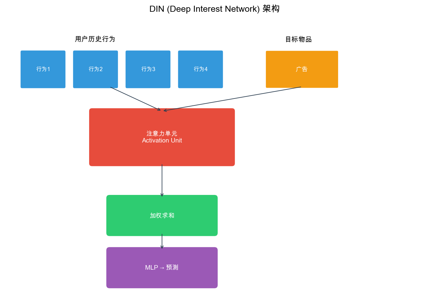
Deep Interest Network (DIN)
DIN 模型架构
DIN 是阿里巴巴在 2018
年提出的深度兴趣网络模型,首次将注意力机制引入到推荐系统的用户兴趣建模中。
核心思想
DIN
的核心创新在于:用户对候选商品的兴趣,应该根据候选商品的不同而动态变化 。传统模型使用固定的用户表示,而
DIN 通过注意力机制,为每个候选商品生成个性化的用户表示。
模型结构
DIN 的整体架构包括以下几个部分:
特征嵌入层 :将稀疏特征转换为密集向量激活单元( Activation
Unit) :计算历史行为与候选商品的注意力权重兴趣提取层 :通过注意力加权聚合历史行为全连接层 :进行最终的特征交互和预测
激活单元设计
DIN 的激活单元是模型的核心组件,负责计算注意力权重:
其中相似度函数
1. 内积注意力
2. 双线性注意力
3. MLP 注意力( DIN 采用)
完整实现
DIN 模型的核心创新在于激活单元( Activation
Unit) 的设计。这个单元负责计算历史行为序列中每个行为项与候选商品之间的注意力权重。与传统注意力机制不同,
DIN 的激活单元使用了 MLP
来学习复杂的交互模式,而不是简单的内积或双线性变换。
激活单元的设计思路 : 1.
多种交互方式 :通过拼接( concat)、相减(
subtract)和逐元素相乘(
multiply)三种方式,充分捕捉候选商品和历史行为之间的交互信息 2.
MLP 学习复杂模式 :使用多层感知机(
MLP)学习这些交互特征的非线性组合,比简单的相似度计算更强大 3.
动态权重分配 :通过 Softmax
归一化,为每个历史行为分配注意力权重,权重高的行为对当前推荐更重要
为什么需要多种交互方式 : - 拼接(
Concat) :保留两个向量的完整信息,让模型学习它们的联合表示 -
相减(
Subtract) :捕捉两个向量的差异,反映候选商品与历史行为的差异程度
- 逐元素相乘(
Multiply) :捕捉两个向量的元素级交互,类似于特征交叉
下面我们实现 DIN
模型的激活单元和完整模型。这个实现展示了如何将注意力机制应用到推荐系统中,以及如何通过动态权重聚合历史行为来建模用户兴趣。
1
2
3
4
5
6
7
8
9
10
11
12
13
14
15
16
17
18
19
20
21
22
23
24
25
26
27
28
29
30
31
32
33
34
35
36
37
38
39
40
41
42
43
44
45
46
47
48
49
50
51
52
53
54
55
56
57
58
59
60
61
62
63
64
65
66
67
68
69
70
71
72
73
74
75
76
77
78
79
80
81
82
83
84
85
86
87
88
89
90
91
92
93
94
95
96
97
98
99
100
101
102
103
104
105
106
107
108
109
110
111
112
113
114
115
116
117
118
119
120
121
122
123
124
125
126
127
128
129
130
131
132
133
134
135
136
137
138
139
140
141
142
143
144
145
146
147
148
149
150
151
152
153
154
155
156
157
158
159
160
161
162
163
164
165
166
167
168
169
170
171
172
173
174
175
176
177
178
179
180
181
182
183
184
185
186
187
188
189
190
191
192
193
194
195
196
197
198
199
200
201
202
203
204
205
206
207
208
209
210
211
212
213
214
215
216
217
218
219
220
221
222
223
224
225
226
227
228
229
230
231
232
233
234
235
236
237
238
239
240
241
242
243
244
245
246
247
248
249
250
251
252
253
254
255
256
257
258
259
260
261
262
263
264
265
266
267
268
269
270
271
272
273
274
275
276
277
278
279
280
281
282
283
284
285
286
287
288
289
import torchimport torch.nn as nnimport torch.nn.functional as Fclass ActivationUnit (nn.Module): """ DIN 的激活单元( Activation Unit) 激活单元是 DIN 模型的核心组件,负责计算历史行为序列中每个行为项 与候选商品之间的注意力权重。 设计要点: 1. 使用多种交互方式(拼接、相减、相乘)捕捉候选商品与历史行为的交互 2. 通过 MLP 学习复杂的非线性交互模式 3. 输出注意力权重,用于加权聚合历史行为 与标准注意力机制的区别: - 标准注意力:使用内积或双线性变换计算相似度 - DIN 激活单元:使用 MLP 学习更复杂的交互模式,表达能力更强 """ def __init__ (self, embedding_dim, hidden_units=[80 , 40 ] ): """ 初始化激活单元 Args: embedding_dim: 嵌入维度,即候选商品和历史行为的向量维度 - 通常设置为 8-64 之间 - 维度越大,表达能力越强,但计算成本也越高 hidden_units: MLP 的隐藏层维度列表,如[80, 40]表示两层 MLP - 第一层:输入维度 -> 80 - 第二层: 80 -> 40 - 输出层: 40 -> 1(注意力分数) - 可以根据数据复杂度调整层数和维度 """ super (ActivationUnit, self).__init__() self.embedding_dim = embedding_dim layers = [] input_dim = embedding_dim * 4 for hidden_dim in hidden_units: layers.append(nn.Linear(input_dim, hidden_dim)) layers.append(nn.ReLU()) input_dim = hidden_dim layers.append(nn.Linear(input_dim, 1 )) self.mlp = nn.Sequential(*layers) def forward (self, query, keys ): """ 计算注意力权重 前向传播流程: 1. 扩展 query 维度,使其与 keys 的每个元素对齐 2. 构建多种交互特征(拼接、相减、相乘) 3. 通过 MLP 计算注意力分数 4. 应用 Softmax 归一化得到注意力权重 Args: query: 候选商品的嵌入向量 shape: [batch_size, embedding_dim] - batch_size: 批次大小 - embedding_dim: 嵌入维度 keys: 历史行为序列的嵌入向量 shape: [batch_size, seq_len, embedding_dim] - seq_len: 历史行为序列长度(如用户最近点击的 20 个商品) Returns: attention_weights: 注意力权重,表示每个历史行为的重要性 shape: [batch_size, seq_len] - 每一行的权重和为 1(经过 Softmax 归一化) - 权重越大,表示该历史行为对当前推荐越重要 """ batch_size, seq_len, embedding_dim = keys.shape query_expanded = query.unsqueeze(1 ).expand(batch_size, seq_len, embedding_dim) concat_feat = torch.cat([query_expanded, keys], dim=-1 ) subtract_feat = query_expanded - keys multiply_feat = query_expanded * keys interaction_feat = torch.cat([concat_feat, subtract_feat, multiply_feat], dim=-1 ) attention_scores = self.mlp(interaction_feat) attention_scores = attention_scores.squeeze(-1 ) attention_weights = F.softmax(attention_scores, dim=1 ) return attention_weights class DIN (nn.Module): """ Deep Interest Network (DIN) 模型 DIN 是阿里巴巴在 2018 年提出的深度兴趣网络,首次将注意力机制引入推荐系统的用户兴趣建模。 核心创新: 1. 动态用户表示:根据候选商品的不同,动态生成个性化的用户表示 2. 注意力机制:通过激活单元计算历史行为的重要性权重 3. 兴趣提取:通过加权聚合历史行为,提取用户对候选商品的兴趣 与传统模型的区别: - 传统模型:使用固定的用户表示(如用户嵌入的平均值) - DIN 模型:为每个候选商品生成不同的用户表示(通过注意力机制) 应用场景: - 电商推荐:根据用户历史浏览/购买行为,推荐相关商品 - 内容推荐:根据用户历史阅读/观看行为,推荐相关内容 - 广告推荐:根据用户历史点击行为,推荐相关广告 """ def __init__ (self, feature_dims, embedding_dim=8 , hidden_units=[200 , 80 , 2 ] ): """ 初始化 DIN 模型 Args: feature_dims: 特征维度字典,定义每个特征的取值范围 - 例如:{'user_id': 1000, 'item_id': 5000, 'category_id': 100} - key: 特征名称 - value: 该特征的唯一值数量(用于创建嵌入层) embedding_dim: 嵌入维度,所有特征共享相同的嵌入维度 - 通常设置为 8-64 之间 - 维度越大,表达能力越强,但参数量也越大 hidden_units: 全连接层的隐藏单元数列表 - 例如:[200, 80, 2] 表示三层全连接网络 - 最后一层通常是 2(二分类)或 1(回归) - 可以根据数据复杂度调整层数和维度 """ super (DIN, self).__init__() self.embedding_dim = embedding_dim self.embeddings = nn.ModuleDict({ name: nn.Embedding(dim, embedding_dim) for name, dim in feature_dims.items() }) self.activation_unit = ActivationUnit(embedding_dim) layers = [] input_dim = sum (feature_dims.values()) * embedding_dim + embedding_dim for hidden_dim in hidden_units[:-1 ]: layers.append(nn.Linear(input_dim, hidden_dim)) layers.append(nn.ReLU()) layers.append(nn.Dropout(0.5 )) input_dim = hidden_dim layers.append(nn.Linear(input_dim, hidden_units[-1 ])) self.fc_layers = nn.Sequential(*layers) def forward (self, x ): """ DIN 模型的前向传播 前向传播流程: 1. 特征嵌入:将稀疏特征转换为密集向量 2. 注意力计算:计算历史行为与候选商品的注意力权重 3. 兴趣提取:通过加权聚合历史行为,提取用户兴趣 4. 特征拼接:拼接用户特征、候选商品特征和加权历史行为 5. 预测输出:通过全连接层输出最终预测 Args: x: 输入特征字典,包含: - user_features: 用户特征, shape 为[batch_size, num_user_features] - 可以是用户 ID 、年龄、性别等 - item_id: 候选商品 ID, shape 为[batch_size] - 当前要预测的商品 - history_items: 历史行为序列, shape 为[batch_size, seq_len] - 用户最近点击/浏览的商品序列 - seq_len 通常是 10-50 之间 Returns: output: 预测分数, shape 为[batch_size, hidden_units[-1]] - 对于二分类任务, hidden_units[-1]=2,输出两个类别的 logits - 对于回归任务, hidden_units[-1]=1,输出预测值 """ batch_size = x['user_features' ].shape[0 ] user_embeds = [] for i, feat_name in enumerate (self.embeddings.keys()): if 'user' in feat_name: user_embeds.append(self.embeddings[feat_name](x['user_features' ][:, i])) user_embed = torch.cat(user_embeds, dim=1 ) if user_embeds else None item_embed = self.embeddings['item_id' ](x['item_id' ]) history_embeds = self.embeddings['item_id' ](x['history_items' ]) attention_weights = self.activation_unit(item_embed, history_embeds) weighted_history = torch.sum ( attention_weights.unsqueeze(-1 ) * history_embeds, dim=1 ) if user_embed is not None : feature_vector = torch.cat([user_embed, item_embed, weighted_history], dim=1 ) else : feature_vector = torch.cat([item_embed, weighted_history], dim=1 ) output = self.fc_layers(feature_vector) return output
DIN 模型的关键技术细节 :
动态用户表示的意义 :传统模型使用固定的用户表示(如用户嵌入的平均值),无法反映用户对不同商品的兴趣差异。
DIN
通过注意力机制,为每个候选商品生成不同的用户表示,更准确地建模用户兴趣。
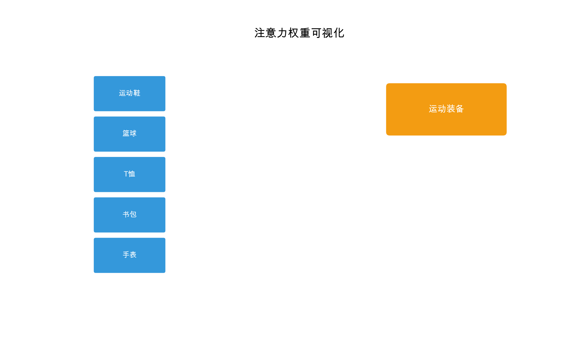
注意力权重的可解释性 :注意力权重直观地反映了不同历史行为的重要性。例如,当推荐手机时,用户最近浏览的手机相关行为会获得更高的注意力权重,而几个月前浏览的服装信息权重较低。
特征交互的设计 :全连接层学习用户特征、候选商品特征和加权历史行为之间的复杂交互。这种设计允许模型捕捉非线性特征关系,提升预测准确性。
参数量分析 :假设有 1000 个用户、 5000
个商品,嵌入维度 8,全连接层[200, 80, 2]。
嵌入层参数量: 1000 × 8 + 5000 × 8 = 48K
激活单元参数量:约(8 × 4)× 80 + 80 × 40 + 40 × 1 ≈ 26K
全连接层参数量:约(48K+8)× 200 + 200 × 80 + 80 × 2 ≈ 10M
总参数量约 10M,相比传统模型(可能需要更多参数)更高效
训练技巧 :
小批量感知正则化 :只对当前批次出现的特征进行正则化,避免全量参数正则化的计算开销数据自适应激活函数( Dice) :替代传统的
PReLU,根据数据分布自适应调整激活函数负采样 :对于大规模推荐系统,使用负采样减少计算量
DIN 的训练技巧
1.
小批量感知正则化( Mini-batch Aware Regularization)
DIN
在处理大规模稀疏特征时,提出了小批量感知正则化方法,避免对全量参数进行正则化:
1
2
3
4
5
6
7
8
9
10
11
12
13
14
15
16
17
18
19
20
21
22
23
class MiniBatchAwareRegularizer : """小批量感知正则化""" def __init__ (self, lambda_reg=1e-5 ): self.lambda_reg = lambda_reg def compute_reg_loss (self, embeddings, batch_samples ): """ Args: embeddings: 嵌入层参数 batch_samples: 当前批次中出现的样本索引 Returns: reg_loss: 正则化损失 """ reg_loss = 0.0 for embedding in embeddings: batch_embeddings = embedding(batch_samples) reg_loss += self.lambda_reg * torch.sum (batch_embeddings ** 2 ) return reg_loss
2. 数据自适应激活函数( Dice)
DIN 提出了数据自适应激活函数 Dice,替代传统的 PReLU:
1
2
3
4
5
6
7
8
9
10
11
12
13
14
15
16
17
18
class Dice (nn.Module): """数据自适应激活函数""" def __init__ (self, input_dim, epsilon=1e-8 ): super (Dice, self).__init__() self.epsilon = epsilon self.alpha = nn.Parameter(torch.zeros(input_dim)) self.bn = nn.BatchNorm1d(input_dim) def forward (self, x ): x_norm = self.bn(x) p = torch.sigmoid(x_norm) return p * x + (1 - p) * self.alpha * x
3. 训练代码示例
1
2
3
4
5
6
7
8
9
10
11
12
13
14
15
16
17
18
19
20
21
22
23
24
25
26
27
28
29
30
31
32
33
34
35
36
37
38
39
40
41
42
43
44
45
46
47
48
49
50
import torch.optim as optimfrom torch.utils.data import DataLoader, Datasetclass DINTrainer : """DIN 模型训练器""" def __init__ (self, model, device='cuda' ): self.model = model.to(device) self.device = device self.optimizer = optim.Adam(model.parameters(), lr=1e-3 ) self.criterion = nn.BCEWithLogitsLoss() self.regularizer = MiniBatchAwareRegularizer() def train_epoch (self, dataloader ): self.model.train() total_loss = 0.0 for batch_idx, batch in enumerate (dataloader): user_features = batch['user_features' ].to(self.device) item_id = batch['item_id' ].to(self.device) history_items = batch['history_items' ].to(self.device) labels = batch['labels' ].to(self.device) x = { 'user_features' : user_features, 'item_id' : item_id, 'history_items' : history_items } logits = self.model(x) loss = self.criterion(logits.squeeze(), labels.float ()) reg_loss = self.regularizer.compute_reg_loss( self.model.embeddings.values(), item_id ) total_loss_batch = loss + reg_loss self.optimizer.zero_grad() total_loss_batch.backward() self.optimizer.step() total_loss += total_loss_batch.item() return total_loss / len (dataloader)
DIN 的优势与局限
优势: 1. 通过注意力机制动态建模用户兴趣 2.
可解释性强,注意力权重直观 3. 在阿里巴巴的广告推荐场景中效果显著
局限: 1. 没有考虑兴趣的演化过程 2.
历史行为序列的建模相对简单 3. 对于长期兴趣和短期兴趣的区分不够明确
Deep Interest Evolution
Network (DIEN)
DIEN 模型架构
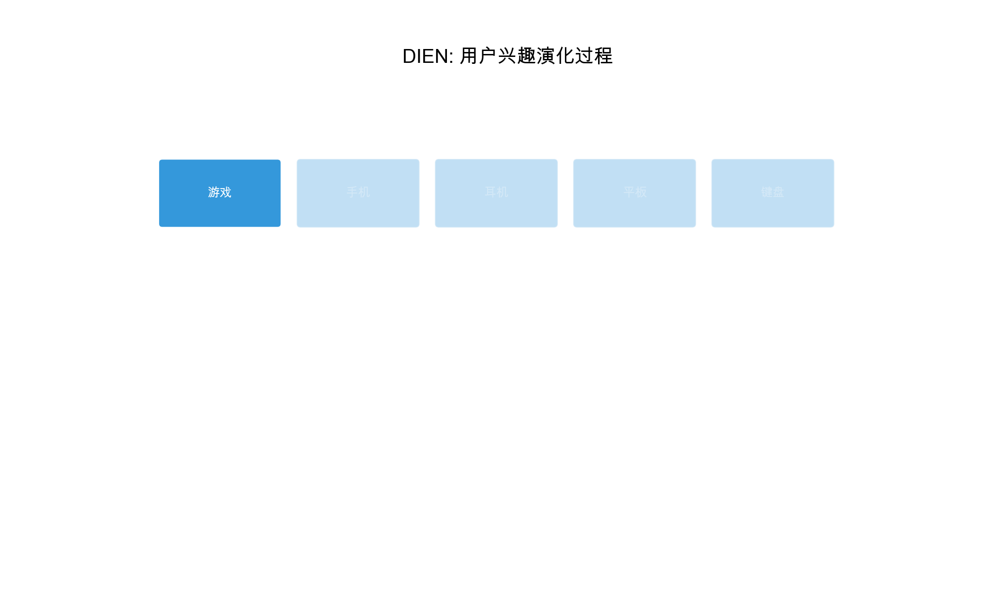
DIEN 在 DIN
的基础上,进一步考虑了用户兴趣的演化过程。基本思路:用户兴趣会随时间演化,需要捕捉兴趣的变化趋势 。
核心创新
DIEN 的主要创新包括:
兴趣提取层( Interest Extractor Layer) :使用 GRU
提取每个时间步的兴趣表示兴趣演化层( Interest Evolution
Layer) :使用带注意力机制的 GRU( AUGRU)捕捉兴趣演化辅助损失( Auxiliary
Loss) :通过预测下一个行为来辅助训练
兴趣提取层
兴趣提取层使用 GRU 从用户行为序列中提取兴趣表示:
其中: -
1
2
3
4
5
6
7
8
9
10
11
12
13
14
15
16
17
18
19
20
21
class InterestExtractor (nn.Module): """兴趣提取层""" def __init__ (self, embedding_dim, hidden_dim ): super (InterestExtractor, self).__init__() self.gru = nn.GRU(embedding_dim, hidden_dim, batch_first=True ) self.hidden_dim = hidden_dim def forward (self, behavior_sequence ): """ Args: behavior_sequence: [batch_size, seq_len, embedding_dim] 行为序列 Returns: interest_sequence: [batch_size, seq_len, hidden_dim] 兴趣序列 """ output, hidden = self.gru(behavior_sequence) return output
兴趣演化层
兴趣演化层是 DIEN 的核心创新,它使用AUGRU( GRU with
Attentive Update Gate) 来捕捉用户兴趣的演化过程。与标准 GRU
不同, AUGRU
使用注意力权重来调整更新门,使得与候选商品相关的兴趣演化更快,不相关的兴趣演化更慢。
AUGRU 的设计动机 : - 标准 GRU
对所有时间步的兴趣都进行相同的更新,无法区分哪些兴趣对当前推荐更重要 -
AUGRU
通过注意力权重动态调整更新门,让模型更关注与候选商品相关的兴趣演化
AUGRU 的更新公式 :
其中: -
关键思想 :如果某个时间步的兴趣与候选商品高度相关(
下面我们实现 AUGRU 和兴趣演化层。这个实现展示了如何将注意力机制集成到
RNN 中,实现动态的兴趣演化建模。
1
2
3
4
5
6
7
8
9
10
11
12
13
14
15
16
17
18
19
20
21
22
23
24
25
26
27
28
29
30
31
32
33
34
35
36
37
38
39
40
41
42
43
44
45
46
47
48
49
50
51
52
53
54
55
56
57
58
59
60
61
62
63
64
65
66
67
68
69
70
71
72
73
74
75
76
77
78
79
80
81
82
83
84
85
86
87
88
89
90
91
92
93
94
95
96
97
98
99
100
101
102
103
104
105
106
107
108
109
110
111
112
113
114
115
116
117
118
119
120
121
122
123
124
125
126
127
128
129
130
131
132
133
134
135
136
137
138
139
140
141
142
143
144
145
146
147
148
149
150
151
152
153
154
155
156
157
158
159
160
161
162
163
164
class AUGRU (nn.Module): """ 带注意力更新门的 GRU( GRU with Attentive Update Gate) AUGRU 是 DIEN 的核心组件,它在标准 GRU 的基础上引入了注意力机制。 通过使用注意力权重调整更新门, AUGRU 能够: 1. 动态控制兴趣的演化速度 2. 让与候选商品相关的兴趣快速演化 3. 让不相关的兴趣缓慢演化,保留历史信息 与标准 GRU 的区别: - 标准 GRU:更新门$u_t$只依赖于当前输入和隐藏状态 - AUGRU:更新门$u_t'$还依赖于注意力权重$a_t$,即$u_t' = a_t \cdot u_t$ """ def __init__ (self, input_dim, hidden_dim ): """ 初始化 AUGRU Args: input_dim: 输入维度,即兴趣表示的维度(来自兴趣提取层) hidden_dim: 隐藏状态维度,即演化后兴趣的维度 - 通常设置为 64-128 之间 - 维度越大,表达能力越强,但计算成本也越高 """ super (AUGRU, self).__init__() self.hidden_dim = hidden_dim self.W_z = nn.Linear(input_dim + hidden_dim, hidden_dim) self.W_r = nn.Linear(input_dim + hidden_dim, hidden_dim) self.W_h = nn.Linear(input_dim + hidden_dim, hidden_dim) def forward (self, input_seq, attention_weights, h_0=None ): """ AUGRU 的前向传播 前向传播流程: 1. 对每个时间步,计算标准 GRU 的更新门、重置门和候选隐藏状态 2. 使用注意力权重调整更新门 3. 基于调整后的更新门更新隐藏状态 Args: input_seq: 输入序列(兴趣序列) shape: [batch_size, seq_len, input_dim] - batch_size: 批次大小 - seq_len: 序列长度(历史行为数量) - input_dim: 输入维度(兴趣表示的维度) attention_weights: 注意力权重(来自激活单元) shape: [batch_size, seq_len] - 每一行表示该样本在不同时间步的注意力权重 - 权重越大,表示该时间步的兴趣与候选商品越相关 h_0: 初始隐藏状态, shape 为[batch_size, hidden_dim] 如果为 None,则初始化为全零向量 Returns: output: 输出序列(演化后的兴趣序列) shape: [batch_size, seq_len, hidden_dim] - 每个时间步的隐藏状态都经过了注意力加权的演化 """ batch_size, seq_len, input_dim = input_seq.shape if h_0 is None : h_0 = torch.zeros(batch_size, self.hidden_dim, device=input_seq.device) outputs = [] h_t = h_0 for t in range (seq_len): x_t = input_seq[:, t, :] a_t = attention_weights[:, t].unsqueeze(1 ) combined = torch.cat([x_t, h_t], dim=1 ) z_t = torch.sigmoid(self.W_z(combined)) r_t = torch.sigmoid(self.W_r(combined)) combined_reset = torch.cat([x_t, r_t * h_t], dim=1 ) h_tilde = torch.tanh(self.W_h(combined_reset)) u_t_prime = a_t * z_t h_t = (1 - u_t_prime) * h_t + u_t_prime * h_tilde outputs.append(h_t) output = torch.stack(outputs, dim=1 ) return output class InterestEvolutionLayer (nn.Module): """兴趣演化层""" def __init__ (self, input_dim, hidden_dim, embedding_dim ): super (InterestEvolutionLayer, self).__init__() self.augru = AUGRU(input_dim, hidden_dim) self.attention_unit = ActivationUnit(embedding_dim) def forward (self, interest_sequence, target_item ): """ Args: interest_sequence: [batch_size, seq_len, hidden_dim] 兴趣序列 target_item: [batch_size, embedding_dim] 目标商品 Returns: evolved_interest: [batch_size, hidden_dim] 演化后的兴趣 """ interest_for_attention = interest_sequence attention_weights = self.attention_unit(target_item, interest_for_attention) evolved_sequence = self.augru(interest_sequence, attention_weights) evolved_interest = evolved_sequence[:, -1 , :] return evolved_interest
辅助损失
DIEN 使用辅助损失来帮助兴趣提取层更好地学习:
其中: -
1
2
3
4
5
6
7
8
9
10
11
12
13
14
15
16
17
18
19
20
21
22
23
24
25
26
27
28
29
30
31
32
class AuxiliaryLoss (nn.Module): """辅助损失""" def __init__ (self ): super (AuxiliaryLoss, self).__init__() def forward (self, interest_sequence, next_behaviors, neg_behaviors ): """ Args: interest_sequence: [batch_size, seq_len, hidden_dim] 兴趣序列 next_behaviors: [batch_size, seq_len, embedding_dim] 下一个行为(正样本) neg_behaviors: [batch_size, seq_len, embedding_dim] 负样本行为 Returns: aux_loss: 辅助损失 """ batch_size, seq_len, hidden_dim = interest_sequence.shape pos_scores = torch.sum (interest_sequence * next_behaviors, dim=-1 ) neg_scores = torch.sum (interest_sequence * neg_behaviors, dim=-1 ) pos_loss = -torch.log(torch.sigmoid(pos_scores) + 1e-8 ) neg_loss = -torch.log(1 - torch.sigmoid(neg_scores) + 1e-8 ) aux_loss = torch.mean(pos_loss + neg_loss) return aux_loss
DIEN 完整实现
DIEN
模型整合了兴趣提取层、兴趣演化层和辅助损失,实现了端到端的用户兴趣演化建模。与
DIN 相比, DIEN
不仅考虑了历史行为的重要性(通过注意力),还考虑了兴趣的时序演化(通过
AUGRU)。
DIEN 的完整流程 : 1.
特征嵌入 :将稀疏特征转换为密集向量 2.
兴趣提取 :使用 GRU 从行为序列中提取每个时间步的兴趣表示
3.
注意力计算 :计算每个时间步的兴趣与候选商品的注意力权重
4. 兴趣演化 :使用 AUGRU 基于注意力权重演化兴趣序列 5.
特征拼接 :拼接用户特征、候选商品特征和演化后的兴趣 6.
预测输出 :通过全连接层输出最终预测
下面我们实现完整的 DIEN 模型。这个实现展示了如何将 GRU
、注意力机制和辅助损失结合起来,实现更强大的用户兴趣建模。
1
2
3
4
5
6
7
8
9
10
11
12
13
14
15
16
17
18
19
20
21
22
23
24
25
26
27
28
29
30
31
32
33
34
35
36
37
38
39
40
41
42
43
44
45
46
47
48
49
50
51
52
53
54
55
56
57
58
59
60
61
62
63
64
65
66
67
68
69
70
71
72
73
74
75
76
77
78
79
80
81
82
83
84
85
86
87
88
89
90
91
92
93
94
95
96
97
98
99
100
101
102
103
104
105
106
107
108
109
110
111
112
113
114
115
116
117
118
119
120
121
122
123
124
125
126
127
128
129
130
131
132
133
134
135
136
137
138
139
140
141
class DIEN (nn.Module): """ Deep Interest Evolution Network (DIEN) DIEN 在 DIN 的基础上,进一步考虑了用户兴趣的演化过程。 核心创新: 1. 兴趣提取层:使用 GRU 提取每个时间步的兴趣表示 2. 兴趣演化层:使用 AUGRU 捕捉兴趣的时序演化 3. 辅助损失:通过预测下一个行为来辅助训练兴趣提取层 与 DIN 的区别: - DIN:静态建模用户兴趣(通过注意力加权历史行为) - DIEN:动态建模用户兴趣演化(通过 GRU 和 AUGRU 捕捉时序变化) """ def __init__ (self, feature_dims, embedding_dim=8 , interest_hidden_dim=64 , evolution_hidden_dim=64 , fc_hidden_units=[200 , 80 , 2 ] ): """ 初始化 DIEN 模型 Args: feature_dims: 特征维度字典,如{'user_id': 1000, 'item_id': 5000} embedding_dim: 嵌入维度,通常设置为 8-64 interest_hidden_dim: 兴趣提取层的隐藏维度( GRU 的输出维度) - 通常设置为 64-128 - 表示每个时间步的兴趣表示的维度 evolution_hidden_dim: 兴趣演化层的隐藏维度( AUGRU 的输出维度) - 通常设置为 64-128 - 表示演化后兴趣的维度 fc_hidden_units: 全连接层的隐藏单元数列表 - 例如:[200, 80, 2] 表示三层全连接网络 - 最后一层通常是 2(二分类)或 1(回归) """ super (DIEN, self).__init__() self.embedding_dim = embedding_dim self.embeddings = nn.ModuleDict({ name: nn.Embedding(dim, embedding_dim) for name, dim in feature_dims.items() }) self.interest_extractor = InterestExtractor(embedding_dim, interest_hidden_dim) self.interest_evolution = InterestEvolutionLayer( interest_hidden_dim, evolution_hidden_dim, embedding_dim ) self.auxiliary_loss = AuxiliaryLoss() layers = [] input_dim = sum (feature_dims.values()) * embedding_dim + evolution_hidden_dim for hidden_dim in fc_hidden_units[:-1 ]: layers.append(nn.Linear(input_dim, hidden_dim)) layers.append(nn.ReLU()) layers.append(nn.Dropout(0.5 )) input_dim = hidden_dim layers.append(nn.Linear(input_dim, fc_hidden_units[-1 ])) self.fc_layers = nn.Sequential(*layers) def forward (self, x, compute_aux_loss=False ): """ DIEN 的前向传播 前向传播流程: 1. 特征嵌入:将稀疏特征转换为密集向量 2. 兴趣提取:使用 GRU 提取兴趣序列 3. 注意力计算:计算兴趣与候选商品的注意力权重 4. 兴趣演化:使用 AUGRU 演化兴趣序列 5. 特征拼接:拼接所有特征 6. 预测输出:通过全连接层输出预测 Args: x: 输入特征字典,包含: - user_features: 用户特征 [batch_size, num_user_features] - item_id: 候选商品 ID [batch_size] - behavior_sequence: 历史行为序列 [batch_size, seq_len] - next_behaviors: 下一个行为(用于辅助损失)[batch_size, seq_len] - neg_behaviors: 负样本行为(用于辅助损失)[batch_size, seq_len] compute_aux_loss: 是否计算辅助损失 - True: 返回主损失和辅助损失 - False: 只返回主预测 Returns: output: 预测输出 [batch_size, fc_hidden_units[-1]] aux_loss: 辅助损失(如果 compute_aux_loss=True) """ output: 预测输出 aux_loss: 辅助损失(如果 compute_aux_loss=True ) """ # 嵌入候选商品 target_item = self.embeddings['item_id'](x['item_id']) # 嵌入行为序列 behavior_sequence = self.embeddings['item_id'](x['history_items']) # 兴趣提取 interest_sequence = self.interest_extractor(behavior_sequence) # 兴趣演化 evolved_interest = self.interest_evolution(interest_sequence, target_item) # 计算辅助损失 aux_loss = None if compute_aux_loss and 'next_behaviors' in x and 'neg_behaviors' in x: next_behaviors = self.embeddings['item_id'](x['next_behaviors']) neg_behaviors = self.embeddings['item_id'](x['neg_behaviors']) aux_loss = self.auxiliary_loss(interest_sequence, next_behaviors, neg_behaviors) # 拼接特征 user_features = self._embed_user_features(x['user_features']) feature_vector = torch.cat([user_features, target_item, evolved_interest], dim=1) # 全连接层 output = self.fc_layers(feature_vector) if compute_aux_loss: return output, aux_loss return output def _embed_user_features(self, user_features): """ 嵌入用户特征""" # 简化实现 return torch.zeros(user_features.shape[0], sum(self.embeddings.keys()) * self.embedding_dim, device=user_features.device)
DIEN 的训练策略
1
2
3
4
5
6
7
8
9
10
11
12
13
14
15
16
17
18
19
20
21
22
23
24
25
26
27
28
29
30
31
32
33
34
35
36
37
38
39
40
41
42
43
44
45
46
47
48
49
50
51
52
53
54
55
56
57
58
59
60
61
class DIENTrainer : """DIEN 训练器""" def __init__ (self, model, device='cuda' , aux_loss_weight=1.0 ): self.model = model.to(device) self.device = device self.aux_loss_weight = aux_loss_weight self.optimizer = optim.Adam(model.parameters(), lr=1e-3 ) self.criterion = nn.BCEWithLogitsLoss() def train_epoch (self, dataloader ): self.model.train() total_loss = 0.0 total_main_loss = 0.0 total_aux_loss = 0.0 for batch in dataloader: item_id = batch['item_id' ].to(self.device) history_items = batch['history_items' ].to(self.device) labels = batch['labels' ].to(self.device) x = { 'item_id' : item_id, 'history_items' : history_items, 'user_features' : batch['user_features' ].to(self.device) } if 'next_behaviors' in batch: x['next_behaviors' ] = batch['next_behaviors' ].to(self.device) x['neg_behaviors' ] = batch['neg_behaviors' ].to(self.device) compute_aux = True else : compute_aux = False if compute_aux: logits, aux_loss = self.model(x, compute_aux_loss=True ) main_loss = self.criterion(logits.squeeze(), labels.float ()) loss = main_loss + self.aux_loss_weight * aux_loss total_main_loss += main_loss.item() total_aux_loss += aux_loss.item() else : logits = self.model(x, compute_aux_loss=False ) loss = self.criterion(logits.squeeze(), labels.float ()) total_main_loss += loss.item() self.optimizer.zero_grad() loss.backward() self.optimizer.step() total_loss += loss.item() return { 'total_loss' : total_loss / len (dataloader), 'main_loss' : total_main_loss / len (dataloader), 'aux_loss' : total_aux_loss / len (dataloader) if total_aux_loss > 0 else 0 }
Deep Session Interest
Network (DSIN)
DSIN 模型架构
DSIN 进一步将用户行为序列划分为多个会话(
Session),认为同一会话内的行为相关性更强,不同会话之间可能存在兴趣转移。
核心创新
DSIN 的主要创新包括:
会话划分 :将用户行为序列划分为多个会话会话内兴趣提取 :使用 Bi-LSTM
提取每个会话内的兴趣会话间兴趣演化 :使用 Transformer
捕捉会话间的兴趣演化目标注意力 :对会话应用目标注意力机制
会话划分
首先需要将用户行为序列划分为会话:
1
2
3
4
5
6
7
8
9
10
11
12
13
14
15
16
17
18
19
20
21
22
23
24
25
26
27
28
29
def split_into_sessions (behavior_sequence, session_gap=30 *60 ): """ 根据时间间隔将会话划分为多个会话 Args: behavior_sequence: list of (item_id, timestamp) tuples session_gap: 会话间隔(秒),默认 30 分钟 Returns: sessions: list of sessions,每个 session 是一个 item_id 列表 """ if len (behavior_sequence) == 0 : return [] sessions = [] current_session = [behavior_sequence[0 ][0 ]] for i in range (1 , len (behavior_sequence)): time_gap = behavior_sequence[i][1 ] - behavior_sequence[i-1 ][1 ] if time_gap > session_gap: sessions.append(current_session) current_session = [behavior_sequence[i][0 ]] else : current_session.append(behavior_sequence[i][0 ]) sessions.append(current_session) return sessions
会话内兴趣提取
使用 Bi-LSTM 提取每个会话内的兴趣:
1
2
3
4
5
6
7
8
9
10
11
12
13
14
15
16
17
18
19
20
21
22
23
24
25
26
27
28
29
30
31
32
33
34
35
36
37
38
class SessionInterestExtractor (nn.Module): """会话内兴趣提取层""" def __init__ (self, embedding_dim, hidden_dim ): super (SessionInterestExtractor, self).__init__() self.bi_lstm = nn.LSTM( embedding_dim, hidden_dim, batch_first=True , bidirectional=True ) self.hidden_dim = hidden_dim def forward (self, session_sequence ): """ Args: session_sequence: [batch_size, num_sessions, session_len, embedding_dim] Returns: session_interests: [batch_size, num_sessions, hidden_dim * 2] """ batch_size, num_sessions, session_len, embedding_dim = session_sequence.shape session_sequence_reshaped = session_sequence.view( batch_size * num_sessions, session_len, embedding_dim ) output, (hidden, _) = self.bi_lstm(session_sequence_reshaped) session_interests = output[:, -1 , :] session_interests = session_interests.view( batch_size, num_sessions, self.hidden_dim * 2 ) return session_interests
会话间兴趣演化
使用 Transformer 捕捉会话间的兴趣演化:
1
2
3
4
5
6
7
8
9
10
11
12
13
14
15
16
17
18
19
20
21
22
23
24
25
26
27
28
29
30
31
32
33
34
35
36
37
38
39
40
41
42
43
44
45
46
47
48
49
50
51
52
53
54
55
56
57
58
59
60
61
class SessionInterestEvolution (nn.Module): """会话间兴趣演化层""" def __init__ (self, input_dim, num_heads=8 , num_layers=2 , dropout=0.1 ): super (SessionInterestEvolution, self).__init__() self.pos_encoding = PositionalEncoding(input_dim, dropout) encoder_layer = nn.TransformerEncoderLayer( d_model=input_dim, nhead=num_heads, dim_feedforward=input_dim * 4 , dropout=dropout, batch_first=True ) self.transformer = nn.TransformerEncoder(encoder_layer, num_layers=num_layers) def forward (self, session_interests ): """ Args: session_interests: [batch_size, num_sessions, input_dim] Returns: evolved_interests: [batch_size, num_sessions, input_dim] """ x = self.pos_encoding(session_interests) evolved_interests = self.transformer(x) return evolved_interests class PositionalEncoding (nn.Module): """位置编码""" def __init__ (self, d_model, dropout=0.1 , max_len=100 ): super (PositionalEncoding, self).__init__() self.dropout = nn.Dropout(p=dropout) pe = torch.zeros(max_len, d_model) position = torch.arange(0 , max_len, dtype=torch.float ).unsqueeze(1 ) div_term = torch.exp(torch.arange(0 , d_model, 2 ).float () * (-math.log(10000.0 ) / d_model)) pe[:, 0 ::2 ] = torch.sin(position * div_term) pe[:, 1 ::2 ] = torch.cos(position * div_term) pe = pe.unsqueeze(0 ) self.register_buffer('pe' , pe) def forward (self, x ): """ Args: x: [batch_size, seq_len, d_model] """ x = x + self.pe[:, :x.size(1 ), :] return self.dropout(x)
目标注意力机制
对会话应用目标注意力:
1
2
3
4
5
6
7
8
9
10
11
12
13
14
15
16
17
18
19
20
21
22
23
24
25
26
class TargetAttention (nn.Module): """目标注意力机制""" def __init__ (self, input_dim ): super (TargetAttention, self).__init__() self.attention_unit = ActivationUnit(input_dim) def forward (self, sessions, target_item ): """ Args: sessions: [batch_size, num_sessions, session_dim] 会话表示 target_item: [batch_size, item_dim] 目标商品 Returns: weighted_sessions: [batch_size, session_dim] 加权后的会话表示 attention_weights: [batch_size, num_sessions] 注意力权重 """ attention_weights = self.attention_unit(target_item, sessions) weighted_sessions = torch.sum ( attention_weights.unsqueeze(-1 ) * sessions, dim=1 ) return weighted_sessions, attention_weights
DSIN 完整实现
1
2
3
4
5
6
7
8
9
10
11
12
13
14
15
16
17
18
19
20
21
22
23
24
25
26
27
28
29
30
31
32
33
34
35
36
37
38
39
40
41
42
43
44
45
46
47
48
49
50
51
52
53
54
55
56
57
58
59
60
61
62
63
64
65
66
67
68
69
70
71
72
73
74
75
76
77
78
79
80
81
82
83
84
85
86
87
88
89
90
91
92
93
94
95
96
97
import mathclass DSIN (nn.Module): """Deep Session Interest Network""" def __init__ (self, feature_dims, embedding_dim=8 , session_hidden_dim=64 , num_heads=8 , num_layers=2 , fc_hidden_units=[200 , 80 , 2 ] ): super (DSIN, self).__init__() self.embedding_dim = embedding_dim self.embeddings = nn.ModuleDict({ name: nn.Embedding(dim, embedding_dim) for name, dim in feature_dims.items() }) self.session_extractor = SessionInterestExtractor( embedding_dim, session_hidden_dim ) session_dim = session_hidden_dim * 2 self.session_evolution = SessionInterestEvolution( session_dim, num_heads, num_layers ) self.target_attention = TargetAttention(session_dim) layers = [] input_dim = sum (feature_dims.values()) * embedding_dim + session_dim for hidden_dim in fc_hidden_units[:-1 ]: layers.append(nn.Linear(input_dim, hidden_dim)) layers.append(nn.ReLU()) layers.append(nn.Dropout(0.5 )) input_dim = hidden_dim layers.append(nn.Linear(input_dim, fc_hidden_units[-1 ])) self.fc_layers = nn.Sequential(*layers) def forward (self, x ): """ Args: x: dict,包含: - item_id: [batch_size] 目标商品 ID - sessions: [batch_size, num_sessions, session_len] 会话序列 - user_features: [batch_size, num_user_features] 用户特征 Returns: output: [batch_size, 1] 预测输出 """ batch_size = x['item_id' ].shape[0 ] target_item = self.embeddings['item_id' ](x['item_id' ]) num_sessions = x['sessions' ].shape[1 ] session_len = x['sessions' ].shape[2 ] session_embeddings = self.embeddings['item_id' ](x['sessions' ]) session_interests = self.session_extractor(session_embeddings) evolved_sessions = self.session_evolution(session_interests) weighted_session, attention_weights = self.target_attention( evolved_sessions, target_item ) user_features = self._embed_user_features(x['user_features' ]) feature_vector = torch.cat([user_features, target_item, weighted_session], dim=1 ) output = self.fc_layers(feature_vector) return output def _embed_user_features (self, user_features ): """嵌入用户特征""" return torch.zeros( user_features.shape[0 ], sum (self.embeddings.keys()) * self.embedding_dim, device=user_features.device )
注意力机制的变种
目标注意力( Target
Attention)
目标注意力是 DIN
系列模型的核心,根据候选商品动态调整历史行为的权重:
1
2
3
4
5
6
7
8
9
10
11
12
13
14
15
16
17
18
19
20
21
22
23
24
25
26
27
28
29
30
31
32
33
34
35
36
37
38
39
40
41
42
43
44
45
46
47
48
49
50
51
52
53
54
55
56
class TargetAttentionVariant (nn.Module): """目标注意力的多种实现""" def __init__ (self, embedding_dim, variant='mlp' ): super (TargetAttentionVariant, self).__init__() self.variant = variant self.embedding_dim = embedding_dim if variant == 'dot' : pass elif variant == 'bilinear' : self.W = nn.Linear(embedding_dim, embedding_dim, bias=False ) elif variant == 'mlp' : self.mlp = nn.Sequential( nn.Linear(embedding_dim * 4 , 80 ), nn.ReLU(), nn.Linear(80 , 40 ), nn.ReLU(), nn.Linear(40 , 1 ) ) def forward (self, query, keys ): """ Args: query: [batch_size, embedding_dim] keys: [batch_size, seq_len, embedding_dim] Returns: attention_weights: [batch_size, seq_len] """ batch_size, seq_len, embedding_dim = keys.shape query_expanded = query.unsqueeze(1 ).expand(batch_size, seq_len, embedding_dim) if self.variant == 'dot' : scores = torch.sum (query_expanded * keys, dim=-1 ) attention_weights = F.softmax(scores, dim=1 ) elif self.variant == 'bilinear' : query_transformed = self.W(query_expanded) scores = torch.sum (query_transformed * keys, dim=-1 ) attention_weights = F.softmax(scores, dim=1 ) elif self.variant == 'mlp' : concat_feat = torch.cat([query_expanded, keys], dim=-1 ) subtract_feat = query_expanded - keys multiply_feat = query_expanded * keys interaction_feat = torch.cat([concat_feat, subtract_feat, multiply_feat], dim=-1 ) scores = self.mlp(interaction_feat).squeeze(-1 ) attention_weights = F.softmax(scores, dim=1 ) return attention_weights
多头注意力( Multi-Head
Attention)
多头注意力允许模型同时关注不同的表示子空间:
1
2
3
4
5
6
7
8
9
10
11
12
13
14
15
16
17
18
19
20
21
22
23
24
25
26
27
28
29
30
31
32
33
34
35
36
37
38
39
40
41
42
43
44
45
46
47
48
49
50
51
52
53
54
55
56
57
58
59
class MultiHeadTargetAttention (nn.Module): """多头目标注意力""" def __init__ (self, embedding_dim, num_heads=8 , dropout=0.1 ): super (MultiHeadTargetAttention, self).__init__() assert embedding_dim % num_heads == 0 self.embedding_dim = embedding_dim self.num_heads = num_heads self.head_dim = embedding_dim // num_heads self.W_q = nn.Linear(embedding_dim, embedding_dim) self.W_k = nn.Linear(embedding_dim, embedding_dim) self.W_v = nn.Linear(embedding_dim, embedding_dim) self.W_o = nn.Linear(embedding_dim, embedding_dim) self.dropout = nn.Dropout(dropout) def forward (self, query, keys, values=None ): """ Args: query: [batch_size, embedding_dim] 目标商品 keys: [batch_size, seq_len, embedding_dim] 历史行为 values: [batch_size, seq_len, embedding_dim] 值(默认与 keys 相同) Returns: output: [batch_size, embedding_dim] 输出 attention_weights: [batch_size, num_heads, seq_len] 注意力权重 """ if values is None : values = keys batch_size = query.shape[0 ] seq_len = keys.shape[1 ] Q = self.W_q(query).view(batch_size, 1 , self.num_heads, self.head_dim).transpose(1 , 2 ) K = self.W_k(keys).view(batch_size, seq_len, self.num_heads, self.head_dim).transpose(1 , 2 ) V = self.W_v(values).view(batch_size, seq_len, self.num_heads, self.head_dim).transpose(1 , 2 ) scores = torch.matmul(Q, K.transpose(-2 , -1 )) / math.sqrt(self.head_dim) attention_weights = F.softmax(scores, dim=-1 ) attention_weights = self.dropout(attention_weights) context = torch.matmul(attention_weights, V) context = context.transpose(1 , 2 ).contiguous().view( batch_size, 1 , self.embedding_dim ) output = self.W_o(context).squeeze(1 ) return output, attention_weights.squeeze(2 )
自注意力( Self-Attention)
自注意力允许序列内的元素相互关注:
1
2
3
4
5
6
7
8
9
10
11
12
13
14
15
16
17
18
19
20
21
22
23
24
25
26
27
28
29
class SelfAttention (nn.Module): """自注意力机制""" def __init__ (self, embedding_dim, num_heads=8 , dropout=0.1 ): super (SelfAttention, self).__init__() self.multi_head_attention = MultiHeadTargetAttention( embedding_dim, num_heads, dropout ) def forward (self, sequence ): """ Args: sequence: [batch_size, seq_len, embedding_dim] Returns: output: [batch_size, seq_len, embedding_dim] """ batch_size, seq_len, embedding_dim = sequence.shape outputs = [] for i in range (seq_len): query = sequence[:, i, :] output_i, _ = self.multi_head_attention(query, sequence) outputs.append(output_i) output = torch.stack(outputs, dim=1 ) return output
位置感知注意力(
Position-Aware Attention)
考虑位置信息的注意力机制:
1
2
3
4
5
6
7
8
9
10
11
12
13
14
15
16
17
18
19
20
21
22
23
24
25
26
27
28
29
30
31
32
33
34
35
36
37
38
39
class PositionAwareAttention (nn.Module): """位置感知注意力""" def __init__ (self, embedding_dim, max_len=100 ): super (PositionAwareAttention, self).__init__() self.embedding_dim = embedding_dim self.pos_embedding = nn.Embedding(max_len, embedding_dim) self.attention_unit = ActivationUnit(embedding_dim) def forward (self, query, keys ): """ Args: query: [batch_size, embedding_dim] keys: [batch_size, seq_len, embedding_dim] Returns: weighted_output: [batch_size, embedding_dim] attention_weights: [batch_size, seq_len] """ batch_size, seq_len, embedding_dim = keys.shape positions = torch.arange(seq_len, device=keys.device).unsqueeze(0 ).expand(batch_size, -1 ) pos_embeds = self.pos_embedding(positions) keys_with_pos = keys + pos_embeds attention_weights = self.attention_unit(query, keys_with_pos) weighted_output = torch.sum ( attention_weights.unsqueeze(-1 ) * keys_with_pos, dim=1 ) return weighted_output, attention_weights
阿里巴巴工业实践
特征工程
在阿里巴巴的推荐系统中,特征工程是模型效果的关键:
1
2
3
4
5
6
7
8
9
10
11
12
13
14
15
16
17
18
19
20
21
22
23
24
25
26
27
28
29
30
31
32
33
34
35
36
37
38
39
40
41
42
43
44
45
46
47
48
49
50
51
52
53
54
55
56
57
58
59
60
61
62
63
class AlibabaFeatureEngineering : """阿里巴巴特征工程实践""" @staticmethod def create_user_features (user_data ): """创建用户特征""" features = {} features['user_id' ] = user_data['user_id' ] features['age' ] = user_data['age' ] features['gender' ] = user_data['gender' ] features['city' ] = user_data['city' ] features['user_click_count' ] = user_data['total_clicks' ] features['user_purchase_count' ] = user_data['total_purchases' ] features['user_avg_price' ] = user_data['avg_purchase_price' ] features['recent_categories' ] = user_data['recent_10_categories' ] features['recent_brands' ] = user_data['recent_10_brands' ] return features @staticmethod def create_item_features (item_data ): """创建商品特征""" features = {} features['item_id' ] = item_data['item_id' ] features['category' ] = item_data['category' ] features['brand' ] = item_data['brand' ] features['price' ] = item_data['price' ] features['item_click_count' ] = item_data['total_clicks' ] features['item_purchase_count' ] = item_data['total_purchases' ] features['item_ctr' ] = item_data['purchase_count' ] / (item_data['click_count' ] + 1 ) features['item_title_embedding' ] = item_data['title_embedding' ] features['item_image_embedding' ] = item_data['image_embedding' ] return features @staticmethod def create_context_features (context_data ): """创建上下文特征""" features = {} features['hour' ] = context_data['hour' ] features['day_of_week' ] = context_data['day_of_week' ] features['is_weekend' ] = context_data['is_weekend' ] features['device_type' ] = context_data['device_type' ] features['os' ] = context_data['os' ] features['browser' ] = context_data['browser' ] return features
训练优化技巧
1. 负采样策略
1
2
3
4
5
6
7
8
9
10
11
12
13
14
15
16
17
18
19
20
21
22
23
24
25
26
27
28
29
30
31
32
33
34
35
36
37
38
39
40
41
42
43
44
45
46
class NegativeSamplingStrategy : """负采样策略""" @staticmethod def random_sampling (item_pool, num_negatives=1 ): """随机负采样""" return np.random.choice(item_pool, size=num_negatives, replace=False ) @staticmethod def popularity_based_sampling (item_popularity, num_negatives=1 , alpha=0.75 ): """ 基于流行度的负采样 Args: item_popularity: 商品流行度字典 num_negatives: 负样本数量 alpha: 采样温度,越小越偏向热门商品 """ popularity_scores = np.array([item_popularity[i] for i in item_popularity.keys()]) probs = popularity_scores ** alpha probs = probs / probs.sum () items = list (item_popularity.keys()) return np.random.choice(items, size=num_negatives, p=probs, replace=False ) @staticmethod def hard_negative_sampling (user_history, candidate_items, num_negatives=1 ): """ 困难负采样:选择用户可能感兴趣但未交互的商品 Args: user_history: 用户历史行为 candidate_items: 候选商品池 num_negatives: 负样本数量 """ negative_candidates = [item for item in candidate_items if item not in user_history] if len (negative_candidates) < num_negatives: return np.random.choice(candidate_items, size=num_negatives, replace=False ) return np.random.choice(negative_candidates, size=num_negatives, replace=False )
2. 学习率调度
1
2
3
4
5
6
7
8
9
10
11
12
13
14
15
16
17
18
19
20
21
22
23
24
25
26
27
class LearningRateScheduler : """学习率调度策略""" @staticmethod def exponential_decay (initial_lr, decay_rate, decay_steps ): """指数衰减""" def scheduler (step ): return initial_lr * (decay_rate ** (step // decay_steps)) return scheduler @staticmethod def warmup_then_decay (initial_lr, warmup_steps, decay_rate ): """预热后衰减""" def scheduler (step ): if step < warmup_steps: return initial_lr * (step / warmup_steps) else : return initial_lr * (decay_rate ** ((step - warmup_steps) // 1000 )) return scheduler @staticmethod def cosine_annealing (initial_lr, T_max, eta_min=0 ): """余弦退火""" def scheduler (step ): return eta_min + (initial_lr - eta_min) * \ (1 + math.cos(math.pi * step / T_max)) / 2 return scheduler
3. 模型集成
1
2
3
4
5
6
7
8
9
10
11
12
13
14
15
16
17
18
19
20
21
22
23
24
25
26
27
28
29
class ModelEnsemble : """模型集成""" def __init__ (self, models, weights=None ): """ Args: models: 模型列表 weights: 权重列表,如果为 None 则平均 """ self.models = models if weights is None : self.weights = [1.0 / len (models)] * len (models) else : assert len (weights) == len (models) total_weight = sum (weights) self.weights = [w / total_weight for w in weights] def predict (self, x ): """集成预测""" predictions = [] for model in self.models: model.eval () with torch.no_grad(): pred = model(x) predictions.append(pred) ensemble_pred = sum (w * p for w, p in zip (self.weights, predictions)) return ensemble_pred
在线服务优化
1. 特征缓存
1
2
3
4
5
6
7
8
9
10
11
12
13
14
15
16
17
18
19
20
21
22
23
24
25
26
27
28
29
30
31
32
33
34
35
36
37
class FeatureCache : """特征缓存""" def __init__ (self, cache_size=10000 , ttl=3600 ): """ Args: cache_size: 缓存大小 ttl: 生存时间(秒) """ self.cache = {} self.cache_size = cache_size self.ttl = ttl self.timestamps = {} def get (self, key ): """获取特征""" if key in self.cache: if time.time() - self.timestamps[key] < self.ttl: return self.cache[key] else : del self.cache[key] del self.timestamps[key] return None def set (self, key, value ): """设置特征""" if len (self.cache) >= self.cache_size: oldest_key = min (self.timestamps.keys(), key=lambda k: self.timestamps[k]) del self.cache[oldest_key] del self.timestamps[oldest_key] self.cache[key] = value self.timestamps[key] = time.time()
2. 模型压缩
1
2
3
4
5
6
7
8
9
10
11
12
13
14
15
16
17
18
19
20
21
22
23
24
25
26
class ModelCompression : """模型压缩""" @staticmethod def quantize_model (model, num_bits=8 ): """模型量化""" quantized_model = torch.quantization.quantize_dynamic( model, {nn.Linear}, dtype=torch.qint8 ) return quantized_model @staticmethod def prune_model (model, pruning_ratio=0.5 ): """模型剪枝""" for module in model.modules(): if isinstance (module, nn.Linear): weight_importance = torch.abs (module.weight.data) threshold = torch.quantile(weight_importance, pruning_ratio) mask = weight_importance > threshold module.weight.data *= mask.float () return model
完整代码实现示例
数据准备
1
2
3
4
5
6
7
8
9
10
11
12
13
14
15
16
17
18
19
20
21
22
23
24
25
26
27
28
29
30
31
32
33
34
35
36
37
38
39
40
41
42
43
44
45
46
47
48
49
50
51
52
53
54
55
56
57
58
import numpy as npimport pandas as pdfrom torch.utils.data import Dataset, DataLoaderclass RecommendationDataset (Dataset ): """推荐系统数据集""" def __init__ (self, data_path, max_seq_len=50 ): """ Args: data_path: 数据路径 max_seq_len: 最大序列长度 """ self.data = pd.read_csv(data_path) self.max_seq_len = max_seq_len self.user_ids = self.data['user_id' ].unique() self.item_ids = self.data['item_id' ].unique() self.user_to_idx = {uid: idx for idx, uid in enumerate (self.user_ids)} self.item_to_idx = {iid: idx for idx, iid in enumerate (self.item_ids)} self.num_users = len (self.user_ids) self.num_items = len (self.item_ids) def __len__ (self ): return len (self.data) def __getitem__ (self, idx ): row = self.data.iloc[idx] user_id = self.user_to_idx[row['user_id' ]] item_id = self.item_to_idx[row['item_id' ]] history_items = eval (row['history_items' ]) history_items = [self.item_to_idx[iid] for iid in history_items if iid in self.item_to_idx] if len (history_items) > self.max_seq_len: history_items = history_items[-self.max_seq_len:] else : history_items = [0 ] * (self.max_seq_len - len (history_items)) + history_items label = row['label' ] return { 'user_id' : torch.LongTensor([user_id]), 'item_id' : torch.LongTensor([item_id]), 'history_items' : torch.LongTensor(history_items), 'label' : torch.FloatTensor([label]) }
训练脚本
1
2
3
4
5
6
7
8
9
10
11
12
13
14
15
16
17
18
19
20
21
22
23
24
25
26
27
28
29
30
31
32
33
34
35
36
37
38
39
40
41
42
43
44
45
46
47
48
49
50
51
52
53
54
55
56
57
58
59
60
61
62
63
64
65
66
67
68
69
70
71
72
73
74
75
76
77
78
79
80
81
82
def train_din_model (model, train_loader, val_loader, num_epochs=10 , device='cuda' ): """训练 DIN 模型""" optimizer = optim.Adam(model.parameters(), lr=1e-3 ) criterion = nn.BCEWithLogitsLoss() scheduler = optim.lr_scheduler.StepLR(optimizer, step_size=3 , gamma=0.5 ) best_val_auc = 0.0 for epoch in range (num_epochs): model.train() train_loss = 0.0 for batch in train_loader: user_id = batch['user_id' ].to(device) item_id = batch['item_id' ].to(device) history_items = batch['history_items' ].to(device) labels = batch['label' ].to(device) x = { 'user_features' : user_id, 'item_id' : item_id, 'history_items' : history_items } logits = model(x) loss = criterion(logits.squeeze(), labels.squeeze()) optimizer.zero_grad() loss.backward() optimizer.step() train_loss += loss.item() val_auc = evaluate_model(model, val_loader, device) print (f'Epoch {epoch+1 } /{num_epochs} ' ) print (f'Train Loss: {train_loss/len (train_loader):.4 f} ' ) print (f'Val AUC: {val_auc:.4 f} ' ) if val_auc > best_val_auc: best_val_auc = val_auc torch.save(model.state_dict(), 'best_din_model.pth' ) scheduler.step() return model def evaluate_model (model, data_loader, device ): """评估模型""" model.eval () all_preds = [] all_labels = [] with torch.no_grad(): for batch in data_loader: user_id = batch['user_id' ].to(device) item_id = batch['item_id' ].to(device) history_items = batch['history_items' ].to(device) labels = batch['label' ].to(device) x = { 'user_features' : user_id, 'item_id' : item_id, 'history_items' : history_items } logits = model(x) preds = torch.sigmoid(logits.squeeze()) all_preds.extend(preds.cpu().numpy()) all_labels.extend(labels.cpu().numpy()) from sklearn.metrics import roc_auc_score auc = roc_auc_score(all_labels, all_preds) return auc
推理服务
1
2
3
4
5
6
7
8
9
10
11
12
13
14
15
16
17
18
19
20
21
22
23
24
25
26
27
28
29
30
31
32
33
34
35
36
37
38
39
40
41
42
43
44
45
46
47
48
49
50
51
52
53
54
55
56
57
58
59
60
61
62
63
64
65
66
67
68
69
70
class InferenceService : """推理服务""" def __init__ (self, model_path, device='cuda' ): self.device = device self.model = self.load_model(model_path) self.model.eval () self.user_to_idx = self.load_dict('user_to_idx.pkl' ) self.item_to_idx = self.load_dict('item_to_idx.pkl' ) def load_model (self, model_path ): """加载模型""" model = DIN(feature_dims={'user_id' : 1000 , 'item_id' : 5000 }, embedding_dim=8 ) model.load_state_dict(torch.load(model_path)) model.to(self.device) return model def predict (self, user_id, item_id, history_items ): """预测""" user_idx = self.user_to_idx.get(user_id, 0 ) item_idx = self.item_to_idx.get(item_id, 0 ) history_indices = [self.item_to_idx.get(iid, 0 ) for iid in history_items] x = { 'user_features' : torch.LongTensor([[user_idx]]).to(self.device), 'item_id' : torch.LongTensor([[item_idx]]).to(self.device), 'history_items' : torch.LongTensor([history_indices]).to(self.device) } with torch.no_grad(): logits = self.model(x) score = torch.sigmoid(logits).item() return score def batch_predict (self, user_ids, item_ids, history_items_list ): """批量预测""" batch_size = len (user_ids) user_indices = [self.user_to_idx.get(uid, 0 ) for uid in user_ids] item_indices = [self.item_to_idx.get(iid, 0 ) for iid in item_ids] max_len = max (len (h) for h in history_items_list) history_tensor = [] for history in history_items_list: history_idx = [self.item_to_idx.get(iid, 0 ) for iid in history] if len (history_idx) < max_len: history_idx = [0 ] * (max_len - len (history_idx)) + history_idx history_tensor.append(history_idx) x = { 'user_features' : torch.LongTensor(user_indices).to(self.device), 'item_id' : torch.LongTensor(item_indices).to(self.device), 'history_items' : torch.LongTensor(history_tensor).to(self.device) } with torch.no_grad(): logits = self.model(x) scores = torch.sigmoid(logits).squeeze().cpu().numpy() return scores
常见问题与解答
Q1: DIN 、 DIEN 、
DSIN 三个模型的主要区别是什么?
A:
三个模型的核心区别在于对用户兴趣建模的层次不同:
DIN :首次引入注意力机制,根据候选商品动态调整历史行为的权重。但它没有考虑兴趣的时间演化。
DIEN :在 DIN 基础上增加了兴趣演化层,使用 GRU 和
AUGRU
捕捉兴趣随时间的变化趋势。通过辅助损失帮助模型更好地学习兴趣表示。
DSIN :进一步将会话概念引入,将用户行为划分为多个会话,使用
Bi-LSTM 提取会话内兴趣,使用 Transformer 捕捉会话间兴趣演化。
选择建议 : - 如果行为序列较短且时间跨度不大,使用
DIN - 如果需要捕捉兴趣演化,使用 DIEN -
如果用户行为有明显的会话划分(如电商浏览),使用 DSIN
Q2:
注意力权重如何解释?权重高的历史行为一定更重要吗?
A:
注意力权重反映了历史行为与候选商品的相关性,但需要注意:
相对重要性 :权重是 softmax
归一化的结果,反映的是相对重要性。如果所有历史行为都与候选商品相关,权重可能相对均匀。
上下文依赖 :权重的高低取决于候选商品。同一个历史行为,对于不同的候选商品,权重可能完全不同。
实际应用 :可以通过可视化注意力权重来理解模型的决策过程,但权重本身不是绝对的"重要性"指标。
1
2
3
4
5
6
7
8
9
10
11
12
13
14
15
16
17
18
19
20
21
def visualize_attention_weights (model, user_history, candidate_items ): """可视化注意力权重""" attention_weights_list = [] for item_id in candidate_items: x = prepare_input(user_history, item_id) with torch.no_grad(): _, attention_weights = model.forward_with_attention(x) attention_weights_list.append(attention_weights.cpu().numpy()) import matplotlib.pyplot as plt import seaborn as sns plt.figure(figsize=(12 , 8 )) sns.heatmap(attention_weights_list, annot=True , fmt='.3f' ) plt.xlabel('History Items' ) plt.ylabel('Candidate Items' ) plt.title('Attention Weights Heatmap' ) plt.show()
Q3:
如何处理序列长度不一致的问题?
A: 有几种常见的处理方法:
填充( Padding) :将短序列填充到固定长度,通常用
0 或特殊 token 。
截断(
Truncation) :将长序列截断到固定长度,可以保留开头、结尾或滑动窗口。
动态批处理 :使用
torch.nn.utils.rnn.pack_padded_sequence
处理变长序列。
1
2
3
4
5
6
7
8
9
10
11
12
13
14
15
16
17
18
19
20
21
22
def handle_variable_length_sequences (sequences, max_len, pad_value=0 ): """处理变长序列""" batch_size = len (sequences) padded_sequences = [] sequence_lengths = [] for seq in sequences: seq_len = len (seq) sequence_lengths.append(min (seq_len, max_len)) if seq_len > max_len: padded_seq = seq[-max_len:] else : padded_seq = [pad_value] * (max_len - seq_len) + seq padded_sequences.append(padded_seq) return torch.LongTensor(padded_sequences), torch.LongTensor(sequence_lengths)
Q4:
辅助损失的作用是什么?如何设置权重?
A: 辅助损失在 DIEN
中用于帮助兴趣提取层更好地学习:
作用 :
提供额外的监督信号
帮助模型学习更有意义的兴趣表示
防止模型过拟合
权重设置 :
通常设置为 0.1 到 1.0 之间
可以通过验证集调优
如果辅助损失过大,可能影响主任务
1 2 3 4 5 6 7 8 9 10 11 class AdaptiveAuxLossWeight : def __init__ (self, initial_weight=1.0 , decay_rate=0.95 ): self.weight = initial_weight self.decay_rate = decay_rate def update (self ): self.weight *= self.decay_rate def get_weight (self ): return self.weight
Q5: 如何加速模型训练?
A: 可以从多个方面优化:
数据加载 :使用多进程数据加载、预取等。
1
2
3
4
5
6
7
8
train_loader = DataLoader( dataset, batch_size=256 , shuffle=True , num_workers=4 , pin_memory=True , prefetch_factor=2 )
混合精度训练 :使用 FP16 加速。
1
2
3
4
5
6
7
8
9
10
11
12
from torch.cuda.amp import autocast, GradScalerscaler = GradScaler() for batch in train_loader: with autocast(): logits = model(x) loss = criterion(logits, labels) scaler.scale(loss).backward() scaler.step(optimizer) scaler.update()
梯度累积 :模拟更大的批次。
1
2
3
4
5
6
7
8
9
10
11
accumulation_steps = 4 optimizer.zero_grad() for i, batch in enumerate (train_loader): loss = compute_loss(batch) loss = loss / accumulation_steps loss.backward() if (i + 1 ) % accumulation_steps == 0 : optimizer.step() optimizer.zero_grad()
Q6: 如何处理冷启动问题?
A: 冷启动是推荐系统的常见挑战:
新用户 :
使用人口统计学特征
利用相似用户的行为
推荐热门商品或多样性商品
新商品 :
使用商品内容特征(标题、图片、类别等)
利用相似商品的信息
探索性推荐
1
2
3
4
5
6
7
8
9
10
11
12
13
14
15
16
17
18
19
20
21
22
class ColdStartHandler : """冷启动处理""" def __init__ (self, model, content_model ): self.model = model self.content_model = content_model def recommend_for_new_user (self, user_features ): """为新用户推荐""" if user_features['history_length' ] == 0 : return self.content_model.recommend(user_features) else : return self.model.recommend(user_features) def recommend_new_item (self, item_features, similar_items ): """推荐新商品""" similar_item_embeddings = self.model.get_item_embeddings(similar_items) new_item_embedding = torch.mean(similar_item_embeddings, dim=0 ) return new_item_embedding
Q7: 如何评估推荐系统的效果?
A: 推荐系统的评估指标包括:
离线指标 :
AUC 、 LogLoss(分类任务)
Precision@K 、 Recall@K 、 NDCG@K(排序任务)
Coverage 、 Diversity(多样性)
在线指标 :
CTR(点击率)
CVR(转化率)
GMV(成交总额)
1
2
3
4
5
6
7
8
9
10
11
12
13
14
15
16
17
18
19
20
21
22
23
24
25
26
def evaluate_recommendation (model, test_data, k=10 ): """评估推荐效果""" metrics = { 'precision' : [], 'recall' : [], 'ndcg' : [] } for user_id, true_items in test_data.items(): recommended_items = model.recommend(user_id, k=k) precision = len (set (recommended_items) & set (true_items)) / k recall = len (set (recommended_items) & set (true_items)) / len (true_items) ndcg = compute_ndcg(recommended_items, true_items) metrics['precision' ].append(precision) metrics['recall' ].append(recall) metrics['ndcg' ].append(ndcg) return { 'precision@{}' .format (k): np.mean(metrics['precision' ]), 'recall@{}' .format (k): np.mean(metrics['recall' ]), 'ndcg@{}' .format (k): np.mean(metrics['ndcg' ]) }
Q8:
模型部署时如何优化推理速度?
A: 推理优化方法:
模型量化 :将 FP32 转为 INT8 。
模型剪枝 :移除不重要的参数。
批处理 :批量处理请求。
特征缓存 :缓存常用特征。
模型蒸馏 :使用小模型替代大模型。
1
2
3
4
5
6
7
8
9
10
11
12
13
14
15
16
17
18
19
20
21
22
23
24
25
26
27
28
29
30
31
32
33
34
35
36
37
38
39
40
41
42
43
44
45
46
class OptimizedInference : """优化的推理服务""" def __init__ (self, model_path ): self.model = torch.quantization.quantize_dynamic( torch.load(model_path), {nn.Linear}, dtype=torch.qint8 ) self.model.eval () self.feature_cache = FeatureCache() self.batch_queue = [] self.batch_size = 32 def predict (self, user_id, item_id, history_items ): """预测(带缓存)""" cache_key = f"{user_id} _{item_id} _{hash (tuple (history_items))} " cached_result = self.feature_cache.get(cache_key) if cached_result is not None : return cached_result result = self._compute_prediction(user_id, item_id, history_items) self.feature_cache.set (cache_key, result) return result def batch_predict (self, requests ): """批量预测""" batch_inputs = self._prepare_batch(requests) with torch.no_grad(): results = self.model(batch_inputs) return results
Q9: 如何处理类别不平衡问题?
A:
类别不平衡在推荐系统中很常见(正样本远少于负样本):
采样策略 :
欠采样:减少负样本
过采样:增加正样本
SMOTE:合成少数类样本
损失函数 :
评估指标 :
1
2
3
4
5
6
7
8
9
10
11
12
13
14
15
16
17
18
19
20
21
22
23
24
25
26
27
class WeightedBCELoss (nn.Module): """加权二分类损失""" def __init__ (self, pos_weight ): super (WeightedBCELoss, self).__init__() self.pos_weight = pos_weight def forward (self, logits, labels ): loss = F.binary_cross_entropy_with_logits( logits, labels, pos_weight=self.pos_weight ) return loss class FocalLoss (nn.Module): """Focal Loss""" def __init__ (self, alpha=1 , gamma=2 ): super (FocalLoss, self).__init__() self.alpha = alpha self.gamma = gamma def forward (self, logits, labels ): bce_loss = F.binary_cross_entropy_with_logits(logits, labels, reduction='none' ) pt = torch.exp(-bce_loss) focal_loss = self.alpha * (1 - pt) ** self.gamma * bce_loss return focal_loss.mean()
Q10: 如何实现实时推荐?
A: 实时推荐需要考虑:
流式处理 :使用 Kafka 、 Flink
等流处理框架。
增量更新 :定期更新用户表示和商品表示。
缓存策略 :缓存热门推荐结果。
异步处理 :将耗时操作异步化。
1
2
3
4
5
6
7
8
9
10
11
12
13
14
15
16
17
18
19
20
21
22
23
24
25
26
27
28
29
30
31
32
33
34
35
36
37
38
39
40
41
42
43
44
45
46
47
48
class RealTimeRecommendation : """实时推荐服务""" def __init__ (self, model, update_interval=300 ): self.model = model self.update_interval = update_interval self.last_update = time.time() self.user_embeddings_cache = {} self.recommendation_cache = {} def update_user_embedding (self, user_id, new_behavior ): """更新用户表示""" if user_id in self.user_embeddings_cache: old_embedding = self.user_embeddings_cache[user_id] new_embedding = self.model.update_user_embedding( old_embedding, new_behavior ) self.user_embeddings_cache[user_id] = new_embedding else : self.user_embeddings_cache[user_id] = \ self.model.get_user_embedding(user_id) def recommend (self, user_id, k=10 ): """实时推荐""" cache_key = f"{user_id} _{k} " if cache_key in self.recommendation_cache: cached_time, cached_result = self.recommendation_cache[cache_key] if time.time() - cached_time < 60 : return cached_result user_embedding = self.user_embeddings_cache.get(user_id) if user_embedding is None : user_embedding = self.model.get_user_embedding(user_id) recommendations = self.model.recommend_from_embedding(user_embedding, k=k) self.recommendation_cache[cache_key] = (time.time(), recommendations) return recommendations
总结
本文深入探讨了深度兴趣网络系列模型( DIN 、 DIEN 、
DSIN)及其在推荐系统中的应用。这些模型通过引入注意力机制,实现了对用户兴趣的动态建模,显著提升了推荐效果。
核心要点总结:
注意力机制 是这些模型的基础,能够根据候选商品动态调整历史行为的重要性。
DIN
首次将注意力机制引入推荐系统,通过激活单元计算注意力权重。
DIEN 在 DIN 基础上增加了兴趣演化层,使用 GRU 和
AUGRU 捕捉兴趣变化。
DSIN 进一步引入会话概念,使用 Bi-LSTM 和
Transformer 分别处理会话内和会话间兴趣。
工业实践 中需要注意特征工程、训练优化、模型部署等多个方面。
常见问题 包括序列处理、冷启动、模型评估等,需要根据具体场景选择合适的解决方案。
随着深度学习技术的不断发展,推荐系统也在持续演进。注意力机制作为其中的重要技术,将继续在推荐系统中发挥重要作用。希望本文能够帮助读者深入理解这些模型,并在实际应用中取得良好效果。