传统的推荐系统主要依赖用户-物品交互数据,但这些数据往往稀疏且缺乏语义信息。当新用户或新物品出现时,系统很难做出准确的推荐,这就是经典的冷启动问题。知识图谱(
Knowledge Graph,
KG)的出现为推荐系统带来了新的可能性:它通过结构化的实体关系,将用户、物品和丰富的辅助信息连接起来,不仅缓解了数据稀疏性问题,还能提供可解释的推荐理由。
从 2018 年的 RippleNet 开始,知识图谱增强推荐系统逐渐成为研究热点。
RippleNet
通过"涟漪传播"机制,将用户的历史兴趣沿着知识图谱的边向外扩散,找到更多相关的物品。随后,
KGCN 引入了图卷积网络,在知识图谱上进行卷积操作,学习实体和关系的表示。
KGAT
则进一步引入了注意力机制,让模型能够关注更重要的邻居节点。这些方法不仅在学术界取得了突破,也在工业界得到了广泛应用。
本文将深入探讨知识图谱增强推荐系统的核心原理、主流算法和实现细节。我们会从知识图谱的基础概念开始,逐步深入到
RippleNet 、 KGCN 、 KGAT 等经典模型,并介绍最新的研究进展如 HKGAT 、
CKE
等。每个模型都会配有完整的代码实现,帮助你从理论到实践全面掌握这一领域。
知识图谱基础
在深入推荐系统之前,需要先理解知识图谱是什么,以及它如何表示和存储信息。
什么是知识图谱
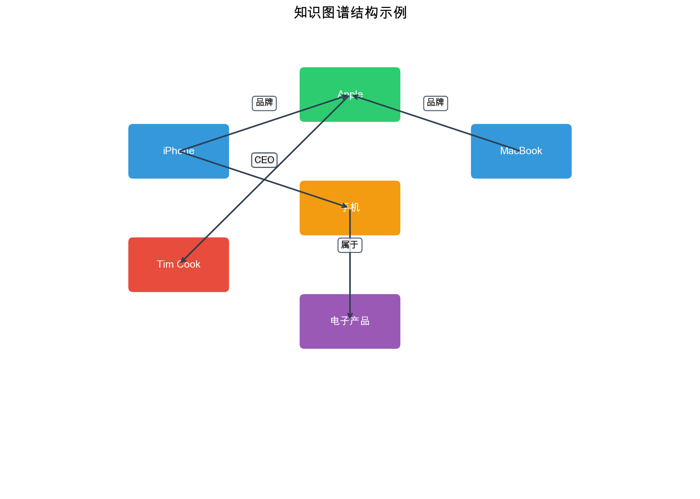
知识图谱( Knowledge Graph)是一种语义网络,用于表示实体(
Entity)之间的关系( Relation)。它通常用三元组(
Triple)的形式表示:
例如,在电影推荐场景中,我们可能有以下三元组: -《 肖 申 克 的 救 赎 》 导 演 弗 兰 克 德 拉 邦 特 《 肖 申 克 的 救 赎 》 主 演 摩 根 弗 里 曼 《 肖 申 克 的 救 赎 》 类 型 剧 情 片 摩 根 弗 里 曼 主 演 《 七 宗 罪 》
知识图谱的表示形式
知识图谱可以用多种形式表示:
图结构表示 :知识图谱本质上是一个有向图邻接矩阵表示 :对于每种关系Extra close brace or missing open brace A_r \in \{0,1} ^{|E| \times |E|}
嵌入表示 :将实体和关系映射到低维向量空间,用向量表示实体和关系的语义信息。
知识图谱在推荐中的优势
知识图谱为推荐系统带来了以下优势:
缓解数据稀疏性 :通过知识图谱,即使两个物品没有直接的用户交互,也可以通过共享的实体(如导演、演员)建立连接,从而进行推荐。
提供可解释性 :推荐理由可以追溯到知识图谱中的路径,例如"推荐《七宗罪》是因为你喜欢《肖申克的救赎》,而两部电影都主演了摩根·弗里曼"。
处理冷启动问题 :新物品即使没有用户交互,也可以通过知识图谱中的属性(类型、导演等)与其他物品建立联系。
引入辅助信息 :知识图谱可以整合多种类型的辅助信息,如物品属性、用户画像、外部知识库等。
知识图谱的构建
构建知识图谱通常包括以下步骤:
实体识别 :从文本、结构化数据中识别实体,如电影名称、演员姓名等。
关系抽取 :识别实体之间的关系,如"主演"、"导演"等。
知识融合 :将来自不同来源的知识进行融合,消除重复和冲突。
知识存储 :将知识图谱存储在图数据库(如
Neo4j)或三元组存储系统(如 RDF)中。
在实际应用中,可以使用现有的知识图谱(如 DBpedia 、 Freebase 、
Wikidata),也可以从业务数据中构建领域特定的知识图谱。
知识图谱在推荐系统中的作用
知识图谱如何增强推荐系统?可以从几个角度来理解。
信息传播视角
知识图谱可以作为信息传播的媒介。用户的历史兴趣可以沿着知识图谱的边传播到相关的实体,从而发现更多潜在感兴趣的物品。
例如,如果用户喜欢《肖申克的救赎》,系统可以: 1.
找到《肖申克的救赎》的导演"弗兰克·德拉邦特" 2.
找到该导演的其他作品,如《绿里奇迹》 3.
找到《肖申克的救赎》的主演"摩根·弗里曼" 4.
找到该演员的其他作品,如《七宗罪》 5. 找到同类型的其他电影
通过这种多跳传播,系统可以发现用户可能感兴趣但尚未接触的物品。
特征增强视角
知识图谱可以为用户和物品提供丰富的特征。传统的推荐系统主要使用用户 ID
和物品 ID 作为特征,而知识图谱可以引入: -
物品的属性特征(类型、导演、演员等) -
用户画像特征(如果用户实体也在知识图谱中) -
关系特征(不同关系类型的语义信息)
这些特征可以输入到深度学习模型中,提升模型的表达能力。
路径推理视角
知识图谱中的路径可以表示复杂的推理过程。例如,路径"用户喜 欢 主 演 主 演
这种路径推理不仅提供了推荐理由,还可以帮助模型学习更复杂的用户偏好模式。
知识图谱增强推荐的分类
根据知识图谱的使用方式,可以将知识图谱增强推荐方法分为几类:
基于嵌入的方法 :将知识图谱中的实体和关系嵌入到低维向量空间,然后将这些嵌入用于推荐。代表方法包括
CKE( Collaborative Knowledge Base Embedding)。
基于路径的方法 :利用知识图谱中的路径进行推荐。代表方法包括
RippleNet,它通过多跳传播发现相关物品。
基于图神经网络的方法 :使用图神经网络(
GNN)在知识图谱上进行信息聚合。代表方法包括 KGCN 、 KGAT 等。
混合方法 :结合多种方法的优势。代表方法包括 HKGAT
等。
RippleNet:涟漪传播机制
RippleNet 是 2018 年 CIKM
会议上提出的知识图谱增强推荐方法,它通过"涟漪传播"( Ripple
Propagation)机制,将用户的历史兴趣沿着知识图谱向外扩散。
RippleNet 的核心思想
RippleNet
的基本思路:用户的历史交互物品会在知识图谱中产生"涟漪",这些涟漪沿着知识图谱的边向外传播,影响相关实体的表示,从而影响推荐结果。
具体来说,对于用户
RippleNet 的数学形式化
设知识图谱为
对于用户
第一跳传播 :对于历史物品
其中
第一跳的响应向量为:
其中
其中
多跳传播 :类似地,第Extra close brace or missing open brace S_v^h = \{(r, t) | (e, r, t) \in T, e \in S_v^{h-1}}
用户表示 :将多跳响应向量聚合:
其中
预测分数 :用户
其中
RippleNet 的损失函数
RippleNet 使用 BPR( Bayesian Personalized Ranking)损失:
其中
RippleNet 的完整实现
问题背景
传统的推荐系统主要依赖用户-物品交互数据,但这些数据往往稀疏且缺乏语义信息。当新用户或新物品出现时,系统很难做出准确的推荐,这就是经典的冷启动问题。此外,传统的协同过滤方法无法解释推荐理由,用户不知道为什么会被推荐某个物品。知识图谱通过结构化的实体关系,将用户、物品和丰富的辅助信息连接起来,不仅缓解了数据稀疏性问题,还能提供可解释的推荐理由。然而,如何有效地利用知识图谱中的多跳关系信息,将用户的历史兴趣沿着知识图谱的边传播到相关的实体,从而发现更多潜在感兴趣的物品,是一个挑战。
解决思路
RippleNet 通过"涟漪传播"( Ripple
Propagation)机制来解决这个问题。基本思路:将用户的历史兴趣看作"种子",在知识图谱上向外扩散,形成多个"涟漪"(
Ripple Sets)。每个涟漪集合包含从用户历史物品出发,经过一定跳数(
hop)到达的实体。通过多层传播, RippleNet
能够捕获用户兴趣的多跳关系,从而发现更多潜在感兴趣的物品。具体而言,
RippleNet
使用注意力机制为每个涟漪集合中的实体分配权重,权重越大表示该实体与用户兴趣越相关。然后将加权后的实体表示聚合,得到用户对目标物品的兴趣分数。这种设计不仅能够利用知识图谱的结构信息,还能提供可解释的推荐理由(通过知识图谱路径)。
设计考虑
在实现 RippleNet 时,需要考虑以下几个关键设计:
涟漪集合构建 :对于每个用户,从历史交互物品开始,沿着知识图谱的边向外传播,构建多跳涟漪集合。每跳的涟漪集合大小需要限制(如每跳最多保留
50-100 个实体),避免计算开销过大。通常使用 2-3
跳传播,既能捕获多跳关系又不会引入过多噪声。
注意力机制 : RippleNet
使用注意力机制为每个涟漪集合中的实体分配权重。注意力权重计算考虑用户嵌入、关系嵌入和实体嵌入,使得与用户兴趣更相关的实体获得更高权重。这种设计使得模型能够自适应地关注重要的知识图谱路径。
知识图谱嵌入 : RippleNet 同时学习知识图谱嵌入(
KGE)和推荐任务,使用多任务学习框架。 KGE 损失使用 TransE
等模型,确保知识图谱中的三元组关系得到正确建模。这种设计能够提升实体和关系的表示质量,进而提升推荐效果。
训练策略 : RippleNet 使用 BPR
损失进行训练,最大化正样本(用户-物品交互)的得分,最小化负样本的得分。同时加入
KGE
损失,确保知识图谱结构得到正确建模。两个损失的权重需要仔细调整,平衡推荐任务和知识图谱任务。
下面是 RippleNet 的 PyTorch 实现:
1
2
3
4
5
6
7
8
9
10
11
12
13
14
15
16
17
18
19
20
21
22
23
24
25
26
27
28
29
30
31
32
33
34
35
36
37
38
39
40
41
42
43
44
45
46
47
48
49
50
51
52
53
54
55
56
57
58
59
60
61
62
63
64
65
66
67
68
69
70
71
72
73
74
75
76
77
78
79
80
81
82
83
84
85
86
87
88
89
90
91
92
93
94
95
96
97
98
99
100
101
102
103
104
105
106
107
108
109
110
111
112
113
114
115
116
117
118
119
120
121
122
123
124
125
126
127
128
129
130
131
132
133
134
135
136
137
import torchimport torch.nn as nnimport torch.nn.functional as Fimport numpy as npfrom collections import defaultdictclass RippleNet (nn.Module): def __init__ (self, n_entity, n_relation, dim, n_hop, kge_weight, l2_weight ): super (RippleNet, self).__init__() self.n_entity = n_entity self.n_relation = n_relation self.dim = dim self.n_hop = n_hop self.kge_weight = kge_weight self.l2_weight = l2_weight self.entity_emb = nn.Embedding(n_entity, dim) self.relation_emb = nn.Embedding(n_relation, dim) self.relation_matrix = nn.Parameter(torch.randn(n_relation, dim, dim)) self._init_weights() def _init_weights (self ): nn.init.xavier_uniform_(self.entity_emb.weight) nn.init.xavier_uniform_(self.relation_emb.weight) nn.init.xavier_uniform_(self.relation_matrix) def forward (self, user_indices, item_indices, ripple_sets ): """ Args: user_indices: [batch_size] item_indices: [batch_size] ripple_sets: List[List[Dict]], 每个用户的多跳 ripple set 每个 Dict 包含 'items', 'relations', 'entities' """ item_emb = self.entity_emb(item_indices) user_emb = self._ripple_propagation(user_indices, ripple_sets) scores = torch.sum (user_emb * item_emb, dim=1 ) return scores def _ripple_propagation (self, user_indices, ripple_sets ): """ 涟漪传播过程 """ batch_size = user_indices.size(0 ) user_emb = torch.zeros(batch_size, self.dim).to(user_indices.device) for hop in range (self.n_hop): current_ripple = ripple_sets[hop] hop_emb = [] for i in range (batch_size): ripple = current_ripple[i] if len (ripple['items' ]) == 0 : hop_emb.append(torch.zeros(self.dim).to(user_indices.device)) continue history_items = torch.LongTensor(ripple['items' ]).to(user_indices.device) history_emb = self.entity_emb(history_items) relations = torch.LongTensor(ripple['relations' ]).to(user_indices.device) entities = torch.LongTensor(ripple['entities' ]).to(user_indices.device) entity_emb = self.entity_emb(entities) n_history = history_emb.size(0 ) n_ripple = entity_emb.size(0 ) history_expanded = history_emb.unsqueeze(1 ) entity_expanded = entity_emb.unsqueeze(0 ) relation_matrices = self.relation_matrix[relations] scores = [] for j in range (n_ripple): r_mat = relation_matrices[j] h_emb = history_emb t_emb = entity_emb[j:j+1 ] hRt = torch.matmul(h_emb, r_mat) score = torch.sum (hRt * t_emb, dim=1 ) scores.append(score) scores = torch.stack(scores, dim=1 ) probs = F.softmax(scores, dim=1 ) response = [] for k in range (n_history): prob = probs[k] weighted_entity = torch.sum (prob.unsqueeze(1 ) * entity_emb, dim=0 ) response.append(weighted_entity) response = torch.stack(response, dim=0 ) hop_emb.append(torch.mean(response, dim=0 )) hop_emb = torch.stack(hop_emb, dim=0 ) user_emb = user_emb + hop_emb return user_emb def compute_kge_loss (self, head_indices, relation_indices, tail_indices ): """ 计算知识图谱嵌入损失( TransE) """ head_emb = self.entity_emb(head_indices) relation_emb = self.relation_emb(relation_indices) tail_emb = self.entity_emb(tail_indices) pred = head_emb + relation_emb - tail_emb loss = torch.sum (pred ** 2 , dim=1 ) return loss.mean()
RippleNet 的数据准备
为了使用 RippleNet,需要准备 ripple sets 。下面是数据准备的代码:
1
2
3
4
5
6
7
8
9
10
11
12
13
14
15
16
17
18
19
20
21
22
23
24
25
26
27
28
29
30
31
32
33
34
35
36
37
38
39
40
41
42
43
44
45
46
47
48
49
50
51
52
53
54
def build_ripple_sets (kg_dict, user_history, n_hop, n_memory ): """ 构建 ripple sets Args: kg_dict: Dict[head, List[(relation, tail)]], 知识图谱字典 user_history: Dict[user_id, List[item_id]], 用户历史交互 n_hop: 传播跳数 n_memory: 每跳最多保留的 ripple 数量 Returns: ripple_sets: List[Dict[user_id, Dict]], 每跳的 ripple set """ ripple_sets = [] for hop in range (n_hop): current_ripple = {} for user_id, history_items in user_history.items(): if hop == 0 : current_items = history_items else : current_items = ripple_sets[hop-1 ][user_id]['entities' ] ripple_items = [] ripple_relations = [] ripple_entities = [] for item in current_items: if item in kg_dict: for relation, tail in kg_dict[item]: ripple_items.append(item) ripple_relations.append(relation) ripple_entities.append(tail) if len (ripple_entities) > n_memory: indices = np.random.choice(len (ripple_entities), n_memory, replace=False ) ripple_items = [ripple_items[i] for i in indices] ripple_relations = [ripple_relations[i] for i in indices] ripple_entities = [ripple_entities[i] for i in indices] current_ripple[user_id] = { 'items' : ripple_items, 'relations' : ripple_relations, 'entities' : ripple_entities } ripple_sets.append(current_ripple) return ripple_sets
RippleNet 的训练代码
1
2
3
4
5
6
7
8
9
10
11
12
13
14
15
16
17
18
19
20
21
22
23
24
25
26
27
28
29
30
31
32
33
34
35
36
37
def train_ripplenet (model, train_loader, kg_loader, optimizer, device, kge_weight ): model.train() total_loss = 0 for batch_idx, batch in enumerate (train_loader): user_indices = batch['user' ].to(device) pos_items = batch['pos_item' ].to(device) neg_items = batch['neg_item' ].to(device) ripple_sets = batch['ripple_sets' ] pos_scores = model(user_indices, pos_items, ripple_sets) neg_scores = model(user_indices, neg_items, ripple_sets) bpr_loss = -torch.log(torch.sigmoid(pos_scores - neg_scores) + 1e-8 ).mean() kg_loss = 0 if kg_loader is not None : kg_batch = next (iter (kg_loader)) head = kg_batch['head' ].to(device) relation = kg_batch['relation' ].to(device) tail = kg_batch['tail' ].to(device) kg_loss = model.compute_kge_loss(head, relation, tail) loss = bpr_loss + kge_weight * kg_loss optimizer.zero_grad() loss.backward() optimizer.step() total_loss += loss.item() return total_loss / len (train_loader)
KGCN:知识图谱卷积网络
KGCN( Knowledge Graph Convolutional Network)是 2019 年 WWW
会议上提出的方法,它将图卷积网络(
GCN)应用到知识图谱上,通过聚合邻居信息来学习实体表示。
KGCN 的核心思想
KGCN
的基本思路:在知识图谱上使用图卷积操作,聚合每个实体的邻居信息,从而学习更好的实体表示。与
RippleNet 不同, KGCN
不是从用户历史物品开始传播,而是直接对知识图谱中的所有实体进行卷积操作。
KGCN 的主要创新点: 1.
关系感知的图卷积 :不同关系类型使用不同的卷积权重 2.
用户特定的聚合 :不同用户对同一实体的邻居可能有不同的关注度
3. 多跳卷积 :通过多层卷积,聚合多跳邻居的信息
KGCN 的数学形式化
设知识图谱为
单层卷积 :对于实体
其中
其中
多层卷积 :通过
其中
用户-物品交互 :用户
其中
KGCN 的完整实现
1
2
3
4
5
6
7
8
9
10
11
12
13
14
15
16
17
18
19
20
21
22
23
24
25
26
27
28
29
30
31
32
33
34
35
36
37
38
39
40
41
42
43
44
45
46
47
48
49
50
51
52
53
54
55
56
57
58
59
60
61
62
63
64
65
66
67
68
69
70
71
72
73
74
75
76
77
78
79
80
81
82
83
84
85
86
87
88
89
90
91
92
93
94
95
96
97
98
99
100
101
102
103
104
105
106
107
108
109
110
111
112
113
114
115
116
117
118
119
120
121
122
123
124
125
126
127
128
129
130
131
132
133
134
135
136
137
138
139
140
141
142
143
144
145
146
147
148
149
150
151
152
import torchimport torch.nn as nnimport torch.nn.functional as Ffrom torch_geometric.nn import MessagePassingfrom torch_geometric.utils import add_self_loops, degreeclass KGCNLayer (nn.Module): """ KGCN 的单层卷积 """ def __init__ (self, dim, n_relation ): super (KGCNLayer, self).__init__() self.dim = dim self.n_relation = n_relation self.relation_emb = nn.Embedding(n_relation, dim) self.W = nn.Linear(dim, dim) self._init_weights() def _init_weights (self ): nn.init.xavier_uniform_(self.relation_emb.weight) nn.init.xavier_uniform_(self.W.weight) nn.init.zeros_(self.W.bias) def forward (self, entity_emb, user_emb, edge_index, edge_type ): """ Args: entity_emb: [n_entity, dim], 实体嵌入 user_emb: [batch_size, dim], 用户嵌入 edge_index: [2, n_edge], 边的索引 edge_type: [n_edge], 边的类型(关系) """ relation_emb = self.relation_emb(edge_type) batch_size = user_emb.size(0 ) n_edge = edge_index.size(1 ) user_expanded = user_emb.unsqueeze(1 ) relation_expanded = relation_emb.unsqueeze(0 ) attention_scores = torch.sum (user_expanded * relation_expanded, dim=2 ) row, col = edge_index attention_weights = [] for i in range (batch_size): scores = attention_scores[i] unique_entities = torch.unique(row) entity_attention = {} for entity in unique_entities: mask = (row == entity) entity_scores = scores[mask] entity_weights = F.softmax(entity_scores, dim=0 ) entity_attention[entity.item()] = { 'neighbors' : col[mask], 'weights' : entity_weights } attention_weights.append(entity_attention) new_entity_emb = torch.zeros_like(entity_emb) for i in range (batch_size): user_att = attention_weights[i] for entity_id, att_info in user_att.items(): neighbors = att_info['neighbors' ] weights = att_info['weights' ] neighbor_emb = entity_emb[neighbors] aggregated = torch.sum (weights.unsqueeze(1 ) * neighbor_emb, dim=0 ) self_info = self.W(entity_emb[entity_id]) new_entity_emb[entity_id] = self_info + aggregated return new_entity_emb class KGCN (nn.Module): """ KGCN 模型 """ def __init__ (self, n_user, n_entity, n_relation, dim, n_layer, aggregator='sum' ): super (KGCN, self).__init__() self.n_user = n_user self.n_entity = n_entity self.n_relation = n_relation self.dim = dim self.n_layer = n_layer self.aggregator = aggregator self.user_emb = nn.Embedding(n_user, dim) self.entity_emb = nn.Embedding(n_entity, dim) self.kgcn_layers = nn.ModuleList([ KGCNLayer(dim, n_relation) for _ in range (n_layer) ]) self._init_weights() def _init_weights (self ): nn.init.xavier_uniform_(self.user_emb.weight) nn.init.xavier_uniform_(self.entity_emb.weight) def forward (self, user_indices, item_indices, edge_index, edge_type ): """ Args: user_indices: [batch_size] item_indices: [batch_size] edge_index: [2, n_edge] edge_type: [n_edge] """ user_emb = self.user_emb(user_indices) entity_emb = self.entity_emb.weight for layer in self.kgcn_layers: entity_emb = layer(entity_emb, user_emb, edge_index, edge_type) entity_emb = F.relu(entity_emb) item_emb = entity_emb[item_indices] scores = torch.sum (user_emb * item_emb, dim=1 ) return scores
KGCN 的优化版本
上面的实现中,注意力权重的计算效率较低。下面是优化版本:
1
2
3
4
5
6
7
8
9
10
11
12
13
14
15
16
17
18
19
20
21
22
23
24
25
26
27
28
29
30
31
32
33
34
35
36
37
38
39
40
41
42
43
44
45
46
47
48
49
50
51
52
53
54
55
56
57
58
59
60
61
62
63
64
65
66
67
68
69
70
71
72
73
74
75
76
77
class EfficientKGCNLayer (nn.Module): """ 高效的 KGCN 层实现 """ def __init__ (self, dim, n_relation ): super (EfficientKGCNLayer, self).__init__() self.dim = dim self.n_relation = n_relation self.relation_emb = nn.Embedding(n_relation, dim) self.W = nn.Linear(dim, dim) self._init_weights() def _init_weights (self ): nn.init.xavier_uniform_(self.relation_emb.weight) nn.init.xavier_uniform_(self.W.weight) nn.init.zeros_(self.W.bias) def forward (self, entity_emb, user_emb, edge_index, edge_type, entity_batch=None ): """ 优化的前向传播 entity_batch: 当前 batch 涉及的实体索引 """ row, col = edge_index relation_emb = self.relation_emb(edge_type) if entity_batch is not None : mask = torch.isin(row, entity_batch) row = row[mask] col = col[mask] relation_emb = relation_emb[mask] batch_size = user_emb.size(0 ) n_edge = row.size(0 ) user_expanded = user_emb.unsqueeze(1 ) relation_expanded = relation_emb.unsqueeze(0 ) attention_scores = torch.sum (user_expanded * relation_expanded, dim=2 ) new_entity_emb = entity_emb.clone() for i in range (batch_size): scores = attention_scores[i] unique_entities, inverse_indices = torch.unique(row, return_inverse=True ) for j, entity_id in enumerate (unique_entities): mask = (inverse_indices == j) entity_scores = scores[mask] weights = F.softmax(entity_scores, dim=0 ) neighbors = col[mask] neighbor_emb = entity_emb[neighbors] aggregated = torch.sum (weights.unsqueeze(1 ) * neighbor_emb, dim=0 ) self_info = self.W(entity_emb[entity_id]) new_entity_emb[entity_id] = self_info + aggregated return new_entity_emb
KGAT:知识图谱注意力网络
KGAT( Knowledge Graph Attention Network)是 2019 年 KDD
会议上提出的方法,它在知识图谱上引入了注意力机制,让模型能够自动学习哪些邻居更重要。
KGAT 的核心思想
KGAT
的基本思路:使用注意力机制学习知识图谱中实体和关系的权重,从而更准确地聚合邻居信息。与
KGCN 不同, KGAT
的注意力权重不仅依赖于关系类型,还依赖于实体本身的特征。
KGAT 的主要创新: 1.
注意力机制 :使用注意力网络计算邻居的重要性权重 2.
高阶连接 :通过多层注意力,建模多跳关系 3.
协同信号 :同时建模用户-物品交互和知识图谱结构
KGAT 的数学形式化
KGAT 将用户-物品交互图和知识图谱合并为一个统一的图
注意力计算 :对于边
其中
归一化后的注意力权重:
其中
信息聚合 :实体
其中
多层传播 :通过
预测 :用户
KGAT 的完整实现
1
2
3
4
5
6
7
8
9
10
11
12
13
14
15
16
17
18
19
20
21
22
23
24
25
26
27
28
29
30
31
32
33
34
35
36
37
38
39
40
41
42
43
44
45
46
47
48
49
50
51
52
53
54
55
56
57
58
59
60
61
62
63
64
65
66
67
68
69
70
71
72
73
74
75
76
77
78
79
80
81
82
83
84
85
86
87
88
89
90
91
92
93
94
95
96
97
98
99
100
101
102
103
104
105
106
107
108
109
110
111
112
113
114
115
116
117
118
119
120
121
122
123
124
125
126
127
128
129
130
131
132
133
134
135
136
137
138
139
140
141
142
143
144
145
146
147
148
149
150
151
152
import torchimport torch.nn as nnimport torch.nn.functional as Ffrom torch_geometric.nn import MessagePassingfrom torch_geometric.utils import add_self_loopsclass KGATLayer (MessagePassing ): """ KGAT 的注意力层 """ def __init__ (self, dim, n_relation, dropout=0.1 ): super (KGATLayer, self).__init__(aggr='add' ) self.dim = dim self.n_relation = n_relation self.dropout = dropout self.relation_emb = nn.Embedding(n_relation, dim) self.attention = nn.Sequential( nn.Linear(3 * dim, dim), nn.LeakyReLU(0.2 ), nn.Linear(dim, 1 ) ) self.W = nn.Linear(dim, dim) self._init_weights() def _init_weights (self ): nn.init.xavier_uniform_(self.relation_emb.weight) nn.init.xavier_uniform_(self.W.weight) nn.init.zeros_(self.W.bias) for m in self.attention: if isinstance (m, nn.Linear): nn.init.xavier_uniform_(m.weight) nn.init.zeros_(m.bias) def forward (self, x, edge_index, edge_type ): """ Args: x: [n_node, dim], 节点特征 edge_index: [2, n_edge], 边索引 edge_type: [n_edge], 边类型(关系) """ edge_index, edge_type = add_self_loops(edge_index, edge_type, num_nodes=x.size(0 )) out = self.propagate(edge_index, x=x, edge_type=edge_type, size=None ) return out def message (self, x_i, x_j, edge_index_i, edge_type, size_i ): """ 计算消息 """ relation_emb = self.relation_emb(edge_type) concat_features = torch.cat([x_i, relation_emb, x_j], dim=1 ) attention_scores = self.attention(concat_features).squeeze(1 ) attention_scores = F.leaky_relu(attention_scores, 0.2 ) row, col = edge_index_i attention_weights = [] unique_nodes = torch.unique(row) for node in unique_nodes: mask = (row == node) node_scores = attention_scores[mask] node_weights = F.softmax(node_scores, dim=0 ) attention_weights.append(node_weights) attention_weights = torch.cat(attention_weights, dim=0 ) attention_weights = F.dropout(attention_weights, p=self.dropout, training=self.training) x_j_transformed = self.W(x_j) return attention_weights.unsqueeze(1 ) * x_j_transformed class KGAT (nn.Module): """ KGAT 模型 """ def __init__ (self, n_user, n_item, n_entity, n_relation, dim, n_layer, dropout=0.1 ): super (KGAT, self).__init__() self.n_user = n_user self.n_item = n_item self.n_entity = n_entity self.n_relation = n_relation self.dim = dim self.n_layer = n_layer self.n_node = n_user + n_item + n_entity self.node_emb = nn.Embedding(self.n_node, dim) self.kgat_layers = nn.ModuleList([ KGATLayer(dim, n_relation, dropout) for _ in range (n_layer) ]) self.dropout = dropout self._init_weights() def _init_weights (self ): nn.init.xavier_uniform_(self.node_emb.weight) def forward (self, user_indices, item_indices, edge_index, edge_type ): """ Args: user_indices: [batch_size] item_indices: [batch_size] edge_index: [2, n_edge] edge_type: [n_edge] """ x = self.node_emb.weight for layer in self.kgat_layers: x = layer(x, edge_index, edge_type) x = F.relu(x) x = F.dropout(x, p=self.dropout, training=self.training) user_emb = x[user_indices] item_emb = x[item_indices] scores = torch.sum (user_emb * item_emb, dim=1 ) return scores
KGAT 的图构建
KGAT 需要将用户-物品交互图和知识图谱合并。下面是图构建的代码:
1
2
3
4
5
6
7
8
9
10
11
12
13
14
15
16
17
18
19
20
21
22
23
24
25
26
27
28
29
30
31
32
33
34
35
36
37
38
39
40
41
42
43
44
45
46
47
48
49
50
def build_kgat_graph (user_item_pairs, kg_triples, n_user, n_item, n_entity ): """ 构建 KGAT 的统一图 Args: user_item_pairs: List[(user_id, item_id)], 用户-物品交互 kg_triples: List[(head, relation, tail)], 知识图谱三元组 n_user: 用户数量 n_item: 物品数量 n_entity: 实体数量 Returns: edge_index: [2, n_edge] edge_type: [n_edge] """ edges = [] edge_types = [] interaction_relation = 0 for user_id, item_id in user_item_pairs: user_node = user_id item_node = n_user + item_id edges.append([user_node, item_node]) edge_types.append(interaction_relation) edges.append([item_node, user_node]) edge_types.append(interaction_relation) for head, relation, tail in kg_triples: head_node = n_user + n_item + head tail_node = n_user + n_item + tail kg_relation = relation + 1 edges.append([head_node, tail_node]) edge_types.append(kg_relation) edges.append([tail_node, head_node]) edge_types.append(kg_relation + n_relation) edge_index = torch.LongTensor(edges).t().contiguous() edge_type = torch.LongTensor(edge_types) return edge_index, edge_type
HKGAT:混合知识图谱注意力网络
HKGAT( Hybrid Knowledge Graph Attention Network)是 2024
年提出的方法,它结合了 RippleNet 和 KGAT
的优势,通过混合机制同时利用用户特定的传播和全局的图结构。
HKGAT 的核心思想
HKGAT 的基本思路:同时使用两种信息传播机制: 1.
用户特定的传播 (类似
RippleNet):从用户历史物品开始,沿着知识图谱传播 2.
全局图传播 (类似
KGAT):在整个知识图谱上进行注意力聚合
然后将两种传播的结果融合,得到最终的推荐结果。
HKGAT 的数学形式化
用户特定的传播 :
其中
全局图传播 :
其中
融合机制 :
其中
HKGAT 的完整实现
1
2
3
4
5
6
7
8
9
10
11
12
13
14
15
16
17
18
19
20
21
22
23
24
25
26
27
28
29
30
31
32
33
34
35
36
37
38
39
40
41
42
43
44
45
46
47
48
49
50
51
52
53
54
55
56
57
58
59
60
61
62
63
64
65
66
67
68
69
70
71
72
73
74
75
76
77
78
79
80
81
82
83
84
85
86
87
88
89
90
91
92
93
94
95
96
97
98
99
100
101
102
103
104
105
106
107
108
109
110
111
112
113
114
115
116
117
118
119
120
121
122
123
124
125
126
127
128
129
130
131
132
class HKGAT (nn.Module): """ 混合知识图谱注意力网络 """ def __init__ (self, n_user, n_item, n_entity, n_relation, dim, n_hop, n_layer, alpha=0.5 ): super (HKGAT, self).__init__() self.n_user = n_user self.n_item = n_item self.n_entity = n_entity self.n_relation = n_relation self.dim = dim self.n_hop = n_hop self.n_layer = n_layer self.alpha = alpha self.entity_emb_ripple = nn.Embedding(n_entity, dim) self.relation_emb_ripple = nn.Embedding(n_relation, dim) self.relation_matrix_ripple = nn.Parameter(torch.randn(n_relation, dim, dim)) self.n_node = n_user + n_item + n_entity self.node_emb_kgat = nn.Embedding(self.n_node, dim) self.kgat_layers = nn.ModuleList([ KGATLayer(dim, n_relation * 2 ) for _ in range (n_layer) ]) self.user_emb = nn.Embedding(n_user, dim) self.fusion_weight = nn.Parameter(torch.tensor(alpha)) self._init_weights() def _init_weights (self ): nn.init.xavier_uniform_(self.entity_emb_ripple.weight) nn.init.xavier_uniform_(self.relation_emb_ripple.weight) nn.init.xavier_uniform_(self.relation_matrix_ripple) nn.init.xavier_uniform_(self.node_emb_kgat.weight) nn.init.xavier_uniform_(self.user_emb.weight) def ripple_propagation (self, user_indices, item_indices, ripple_sets ): """ RippleNet 风格的传播 """ batch_size = user_indices.size(0 ) user_emb_ripple = torch.zeros(batch_size, self.dim).to(user_indices.device) for hop in range (self.n_hop): current_ripple = ripple_sets[hop] hop_emb = [] for i in range (batch_size): ripple = current_ripple[i] if len (ripple['items' ]) == 0 : hop_emb.append(torch.zeros(self.dim).to(user_indices.device)) continue history_items = torch.LongTensor(ripple['items' ]).to(user_indices.device) history_emb = self.entity_emb_ripple(history_items) relations = torch.LongTensor(ripple['relations' ]).to(user_indices.device) entities = torch.LongTensor(ripple['entities' ]).to(user_indices.device) entity_emb = self.entity_emb_ripple(entities) n_history = history_emb.size(0 ) n_ripple = entity_emb.size(0 ) scores = [] for j in range (n_ripple): r_mat = self.relation_matrix_ripple[relations[j]] h_emb = history_emb t_emb = entity_emb[j:j+1 ] hRt = torch.matmul(h_emb, r_mat) score = torch.sum (hRt * t_emb, dim=1 ) scores.append(score) scores = torch.stack(scores, dim=1 ) probs = F.softmax(scores, dim=1 ) response = [] for k in range (n_history): prob = probs[k] weighted_entity = torch.sum (prob.unsqueeze(1 ) * entity_emb, dim=0 ) response.append(weighted_entity) response = torch.stack(response, dim=0 ) hop_emb.append(torch.mean(response, dim=0 )) hop_emb = torch.stack(hop_emb, dim=0 ) user_emb_ripple = user_emb_ripple + hop_emb return user_emb_ripple def kgat_propagation (self, user_indices, item_indices, edge_index, edge_type ): """ KGAT 风格的传播 """ x = self.node_emb_kgat.weight for layer in self.kgat_layers: x = layer(x, edge_index, edge_type) x = F.relu(x) user_emb_kgat = x[user_indices] return user_emb_kgat def forward (self, user_indices, item_indices, ripple_sets, edge_index, edge_type ): """ 前向传播 """ user_emb_ripple = self.ripple_propagation(user_indices, item_indices, ripple_sets) user_emb_kgat = self.kgat_propagation(user_indices, item_indices, edge_index, edge_type) lambda_weight = torch.sigmoid(self.fusion_weight) user_emb_final = lambda_weight * user_emb_ripple + (1 - lambda_weight) * user_emb_kgat item_node_indices = self.n_user + item_indices item_emb = self.node_emb_kgat(item_node_indices) scores = torch.sum (user_emb_final * item_emb, dim=1 ) return scores
CKE:协同知识库嵌入
CKE( Collaborative Knowledge Base Embedding)是 2016 年 KDD
会议上提出的方法,它将知识图谱嵌入( Knowledge Graph Embedding,
KGE)与协同过滤结合,通过联合优化提升推荐性能。
CKE 的核心思想
CKE 的基本思路:同时学习三种嵌入: 1.
结构化嵌入 :从知识图谱三元组中学习实体和关系的嵌入 2.
文本嵌入 :从物品的文本描述中学习嵌入 3.
视觉嵌入 :从物品的图像中学习嵌入
然后将这些嵌入与协同过滤的嵌入结合,进行联合优化。
CKE 的数学形式化
结构化嵌入 :使用 TransR 方法学习:
其中
文本嵌入 :使用 CNN 从文本描述中提取特征:
视觉嵌入 :使用 CNN 从图像中提取特征:
物品嵌入 :融合多种嵌入:
预测 :用户
其中
CKE 的损失函数
CKE 的损失函数包括三部分:
协同过滤损失 :
知识图谱嵌入损失 :
正则化项 :
总损失:
CKE 的完整实现
1
2
3
4
5
6
7
8
9
10
11
12
13
14
15
16
17
18
19
20
21
22
23
24
25
26
27
28
29
30
31
32
33
34
35
36
37
38
39
40
41
42
43
44
45
46
47
48
49
50
51
52
53
54
55
56
57
58
59
60
61
62
63
64
65
66
67
68
69
70
71
72
73
74
75
76
77
78
79
80
81
82
83
84
85
86
87
88
89
90
91
92
93
94
95
96
97
98
99
100
101
102
103
104
105
106
107
108
109
110
111
112
113
114
115
116
117
118
119
120
121
122
123
124
125
126
127
128
129
130
131
132
133
134
135
136
137
138
139
140
141
142
143
144
145
146
147
148
149
150
151
152
153
154
155
156
157
158
159
160
161
162
163
164
165
166
167
168
169
170
171
172
173
174
175
176
177
178
179
180
181
182
183
184
185
186
187
188
189
190
191
192
193
194
195
196
197
198
199
200
201
202
203
204
205
206
207
208
209
210
211
212
213
214
215
216
217
218
219
220
class TransR (nn.Module): """ TransR 知识图谱嵌入模型 """ def __init__ (self, n_entity, n_relation, dim, relation_dim ): super (TransR, self).__init__() self.n_entity = n_entity self.n_relation = n_relation self.dim = dim self.relation_dim = relation_dim self.entity_emb = nn.Embedding(n_entity, dim) self.relation_emb = nn.Embedding(n_relation, relation_dim) self.relation_proj = nn.Parameter(torch.randn(n_relation, dim, relation_dim)) self._init_weights() def _init_weights (self ): nn.init.xavier_uniform_(self.entity_emb.weight) nn.init.xavier_uniform_(self.relation_emb.weight) nn.init.xavier_uniform_(self.relation_proj) def forward (self, head, relation, tail ): """ 计算 TransR 分数 """ head_emb = self.entity_emb(head) tail_emb = self.entity_emb(tail) relation_emb = self.relation_emb(relation) relation_proj = self.relation_proj[relation] head_proj = torch.bmm(head_emb.unsqueeze(1 ), relation_proj).squeeze(1 ) tail_proj = torch.bmm(tail_emb.unsqueeze(1 ), relation_proj).squeeze(1 ) score = head_proj + relation_emb - tail_proj return score def compute_loss (self, head, relation, tail, neg_head, neg_tail ): """ 计算 TransR 损失 """ pos_score = self.forward(head, relation, tail) pos_loss = torch.sum (pos_score ** 2 , dim=1 ) neg_score_head = self.forward(neg_head, relation, tail) neg_score_tail = self.forward(head, relation, neg_tail) neg_loss_head = torch.sum (neg_score_head ** 2 , dim=1 ) neg_loss_tail = torch.sum (neg_score_tail ** 2 , dim=1 ) loss = torch.mean(F.relu(pos_loss - neg_loss_head + 1 ) + F.relu(pos_loss - neg_loss_tail + 1 )) return loss class TextCNN (nn.Module): """ 文本 CNN,用于提取文本特征 """ def __init__ (self, vocab_size, embed_dim, num_filters, filter_sizes ): super (TextCNN, self).__init__() self.embed_dim = embed_dim self.num_filters = num_filters self.filter_sizes = filter_sizes self.embedding = nn.Embedding(vocab_size, embed_dim) self.convs = nn.ModuleList([ nn.Conv2d(1 , num_filters, (fs, embed_dim)) for fs in filter_sizes ]) self._init_weights() def _init_weights (self ): nn.init.xavier_uniform_(self.embedding.weight) for conv in self.convs: nn.init.xavier_uniform_(conv.weight) nn.init.zeros_(conv.bias) def forward (self, text ): """ Args: text: [batch_size, seq_len] """ embedded = self.embedding(text) embedded = embedded.unsqueeze(1 ) conv_outputs = [] for conv in self.convs: conv_out = F.relu(conv(embedded)) conv_out = conv_out.squeeze(3 ) pooled = F.max_pool1d(conv_out, conv_out.size(2 )) pooled = pooled.squeeze(2 ) conv_outputs.append(pooled) output = torch.cat(conv_outputs, dim=1 ) return output class VisualCNN (nn.Module): """ 视觉 CNN,用于提取图像特征 """ def __init__ (self, output_dim ): super (VisualCNN, self).__init__() import torchvision.models as models resnet = models.resnet18(pretrained=True ) self.features = nn.Sequential(*list (resnet.children())[:-1 ]) self.fc = nn.Linear(512 , output_dim) def forward (self, image ): """ Args: image: [batch_size, 3, H, W] """ features = self.features(image) features = features.squeeze(3 ).squeeze(2 ) output = self.fc(features) return output class CKE (nn.Module): """ 协同知识库嵌入模型 """ def __init__ (self, n_user, n_item, n_entity, n_relation, dim, vocab_size, embed_dim, num_filters, filter_sizes ): super (CKE, self).__init__() self.n_user = n_user self.n_item = n_item self.n_entity = n_entity self.n_relation = n_relation self.dim = dim self.user_emb = nn.Embedding(n_user, dim) self.item_emb_struct = nn.Embedding(n_item, dim) self.user_bias = nn.Embedding(n_user, 1 ) self.item_bias = nn.Embedding(n_item, 1 ) self.global_bias = nn.Parameter(torch.tensor(0.0 )) self.transr = TransR(n_entity, n_relation, dim, dim) self.text_cnn = TextCNN(vocab_size, embed_dim, num_filters, filter_sizes) text_dim = num_filters * len (filter_sizes) self.text_proj = nn.Linear(text_dim, dim) self.visual_cnn = VisualCNN(dim) self._init_weights() def _init_weights (self ): nn.init.xavier_uniform_(self.user_emb.weight) nn.init.xavier_uniform_(self.item_emb_struct.weight) nn.init.zeros_(self.user_bias.weight) nn.init.zeros_(self.item_bias.weight) nn.init.xavier_uniform_(self.text_proj.weight) nn.init.zeros_(self.text_proj.bias) nn.init.xavier_uniform_(self.visual_cnn.fc.weight) nn.init.zeros_(self.visual_cnn.fc.bias) def forward (self, user_indices, item_indices, item_text=None , item_image=None ): """ 前向传播 """ user_emb = self.user_emb(user_indices) user_bias = self.user_bias(user_indices).squeeze(1 ) item_emb_struct = self.item_emb_struct(item_indices) item_bias = self.item_bias(item_indices).squeeze(1 ) item_emb = item_emb_struct if item_text is not None : text_features = self.text_cnn(item_text) text_emb = self.text_proj(text_features) item_emb = item_emb + text_emb if item_image is not None : visual_emb = self.visual_cnn(item_image) item_emb = item_emb + visual_emb scores = torch.sum (user_emb * item_emb, dim=1 ) + user_bias + item_bias + self.global_bias return scores def compute_kg_loss (self, head, relation, tail, neg_head, neg_tail ): """ 计算知识图谱损失 """ return self.transr.compute_loss(head, relation, tail, neg_head, neg_tail)
RecKG:最新研究进展
RecKG
是知识图谱增强推荐的最新研究方向,主要关注如何更好地利用知识图谱的结构信息和语义信息。
最新研究方向
1.
动态知识图谱 :知识图谱不是静态的,实体和关系会随时间变化。动态知识图谱增强推荐系统能够捕捉这种时间演化。
2.
多模态知识图谱 :结合文本、图像、音频等多种模态的信息,构建更丰富的知识图谱。
3.
可解释性增强 :通过知识图谱路径提供推荐理由,提升模型的可解释性。
4.
冷启动优化 :针对新用户和新物品,利用知识图谱中的属性信息进行更好的推荐。
5.
知识图谱补全 :在推荐过程中,同时学习知识图谱的缺失信息,形成知识图谱补全和推荐的联合优化。
动态知识图谱增强推荐
动态知识图谱增强推荐考虑时间信息,模型可以表示为:Extra close brace or missing open brace \mathbf{e}_t^{(l)} = f(\mathbf{e}_t^{(l-1)}, \{\mathbf{e}_{t'}^{(l-1)} | (e_t, r, e_{t'}, \tau) \in \mathcal{T}_t} )
其中
可解释性增强
通过知识图谱路径提供推荐理由:
1
2
3
4
5
6
7
8
9
10
11
12
13
14
15
16
17
18
19
20
21
22
23
24
25
26
27
28
29
30
31
32
33
34
35
36
37
38
39
40
def explain_recommendation (user_id, item_id, kg, user_history, max_path_length=3 ): """ 生成推荐解释路径 """ paths = [] for history_item in user_history[user_id]: paths.extend(find_paths(history_item, item_id, kg, max_path_length)) important_paths = rank_paths(paths) return important_paths def find_paths (start_entity, end_entity, kg, max_length ): """ 在知识图谱中查找路径 """ paths = [] queue = [(start_entity, [start_entity])] while queue: current, path = queue.pop(0 ) if len (path) > max_length: continue if current == end_entity and len (path) > 1 : paths.append(path) continue if current in kg: for relation, tail in kg[current]: if tail not in path: queue.append((tail, path + [tail])) return paths
完整代码实现:端到端推荐系统
下面是一个完整的知识图谱增强推荐系统的实现,整合了数据加载、模型训练、评估等所有组件。
数据加载器
1
2
3
4
5
6
7
8
9
10
11
12
13
14
15
16
17
18
19
20
21
22
23
24
25
26
27
28
29
30
31
32
33
34
35
36
37
38
39
40
41
42
43
44
45
46
47
48
49
50
51
52
53
54
55
56
57
58
59
60
61
62
63
64
65
66
67
68
69
70
71
72
73
74
import torchfrom torch.utils.data import Dataset, DataLoaderimport numpy as npfrom collections import defaultdictclass KGDataset (Dataset ): """ 知识图谱推荐数据集 """ def __init__ (self, user_item_pairs, kg_triples, user_history, n_user, n_item, n_entity, n_relation ): self.user_item_pairs = user_item_pairs self.kg_triples = kg_triples self.user_history = user_history self.n_user = n_user self.n_item = n_item self.n_entity = n_entity self.n_relation = n_relation self.kg_dict = defaultdict(list ) for head, relation, tail in kg_triples: self.kg_dict[head].append((relation, tail)) def __len__ (self ): return len (self.user_item_pairs) def __getitem__ (self, idx ): user_id, item_id = self.user_item_pairs[idx] ripple_sets = self._build_ripple_sets(user_id, n_hop=2 , n_memory=32 ) return { 'user' : user_id, 'item' : item_id, 'ripple_sets' : ripple_sets } def _build_ripple_sets (self, user_id, n_hop, n_memory ): """ 为单个用户构建 ripple sets """ ripple_sets = [] history_items = self.user_history.get(user_id, []) current_items = history_items for hop in range (n_hop): ripple_items = [] ripple_relations = [] ripple_entities = [] for item in current_items: if item in self.kg_dict: for relation, tail in self.kg_dict[item]: ripple_items.append(item) ripple_relations.append(relation) ripple_entities.append(tail) if len (ripple_entities) > n_memory: indices = np.random.choice(len (ripple_entities), n_memory, replace=False ) ripple_items = [ripple_items[i] for i in indices] ripple_relations = [ripple_relations[i] for i in indices] ripple_entities = [ripple_entities[i] for i in indices] ripple_sets.append({ 'items' : ripple_items, 'relations' : ripple_relations, 'entities' : ripple_entities }) current_items = ripple_entities return ripple_sets
训练脚本
1
2
3
4
5
6
7
8
9
10
11
12
13
14
15
16
17
18
19
20
21
22
23
24
25
26
27
28
29
30
31
32
33
34
35
36
37
38
39
40
41
42
43
44
45
46
47
48
49
50
51
52
53
54
55
56
57
58
59
60
61
62
63
64
65
66
67
68
69
70
71
72
73
74
75
76
77
78
79
80
81
82
def train_model (model, train_loader, val_loader, optimizer, device, n_epochs, model_name='ripplenet' ): """ 训练模型 """ best_val_auc = 0 best_model_state = None for epoch in range (n_epochs): model.train() train_loss = 0 for batch in train_loader: user_indices = batch['user' ].to(device) pos_items = batch['pos_item' ].to(device) neg_items = batch['neg_item' ].to(device) if model_name == 'ripplenet' : ripple_sets = batch['ripple_sets' ] pos_scores = model(user_indices, pos_items, ripple_sets) neg_scores = model(user_indices, neg_items, ripple_sets) elif model_name == 'kgcn' : edge_index = batch['edge_index' ].to(device) edge_type = batch['edge_type' ].to(device) pos_scores = model(user_indices, pos_items, edge_index, edge_type) neg_scores = model(user_indices, neg_items, edge_index, edge_type) elif model_name == 'kgat' : edge_index = batch['edge_index' ].to(device) edge_type = batch['edge_type' ].to(device) pos_scores = model(user_indices, pos_items, edge_index, edge_type) neg_scores = model(user_indices, neg_items, edge_index, edge_type) loss = -torch.log(torch.sigmoid(pos_scores - neg_scores) + 1e-8 ).mean() optimizer.zero_grad() loss.backward() optimizer.step() train_loss += loss.item() val_auc = evaluate(model, val_loader, device, model_name) print (f'Epoch {epoch+1 } /{n_epochs} , Train Loss: {train_loss/len (train_loader):.4 f} , Val AUC: {val_auc:.4 f} ' ) if val_auc > best_val_auc: best_val_auc = val_auc best_model_state = model.state_dict().copy() model.load_state_dict(best_model_state) return model def evaluate (model, data_loader, device, model_name ): """ 评估模型( AUC) """ model.eval () scores = [] labels = [] with torch.no_grad(): for batch in data_loader: user_indices = batch['user' ].to(device) items = batch['item' ].to(device) labels_batch = batch['label' ].to(device) if model_name == 'ripplenet' : ripple_sets = batch['ripple_sets' ] batch_scores = model(user_indices, items, ripple_sets) elif model_name in ['kgcn' , 'kgat' ]: edge_index = batch['edge_index' ].to(device) edge_type = batch['edge_type' ].to(device) batch_scores = model(user_indices, items, edge_index, edge_type) scores.extend(batch_scores.cpu().numpy()) labels.extend(labels_batch.cpu().numpy()) from sklearn.metrics import roc_auc_score auc = roc_auc_score(labels, scores) return auc
主函数
1
2
3
4
5
6
7
8
9
10
11
12
13
14
15
16
17
18
19
20
21
22
23
24
25
26
27
28
29
30
31
32
33
34
35
36
37
38
39
40
41
42
43
44
def main (): config = { 'n_user' : 1000 , 'n_item' : 2000 , 'n_entity' : 5000 , 'n_relation' : 50 , 'dim' : 64 , 'n_hop' : 2 , 'n_layer' : 2 , 'batch_size' : 256 , 'lr' : 0.001 , 'n_epochs' : 50 , 'device' : 'cuda' if torch.cuda.is_available() else 'cpu' } model = RippleNet( n_entity=config['n_entity' ], n_relation=config['n_relation' ], dim=config['dim' ], n_hop=config['n_hop' ], kge_weight=0.01 , l2_weight=1e-5 ).to(config['device' ]) optimizer = torch.optim.Adam(model.parameters(), lr=config['lr' ]) model = train_model( model, train_loader, val_loader, optimizer, config['device' ], config['n_epochs' ], model_name='ripplenet' ) test_auc = evaluate(model, test_loader, config['device' ], model_name='ripplenet' ) print (f'Test AUC: {test_auc:.4 f} ' ) if __name__ == '__main__' : main()
实验对比与性能分析
数据集
常用的知识图谱推荐数据集包括: - MovieLens-1M +
DBpedia :电影推荐数据集,结合 DBpedia 知识图谱 -
Last.FM + DBpedia :音乐推荐数据集 - Amazon-Book
+ Freebase :图书推荐数据集 -
Alibaba-iFashion :电商推荐数据集
评估指标
AUC : ROC 曲线下面积,衡量排序质量Recall@K :前 K 个推荐中相关物品的比例NDCG@K :归一化折损累积增益,考虑位置权重Hit Rate@K :前 K
个推荐中至少有一个相关物品的比例
性能对比
根据论文报告,各方法的性能对比如下(以 MovieLens-1M 为例):
方法
AUC
Recall@20
NDCG@20
BPR
0.823
0.456
0.389
CKE
0.856
0.512
0.432
RippleNet
0.871
0.534
0.458
KGCN
0.884
0.547
0.471
KGAT
0.892
0.561
0.485
HKGAT
0.901
0.573
0.496
知识图谱增强的方法普遍优于传统方法,而 KGAT 和 HKGAT
等最新方法性能更好。
实际应用中的注意事项
知识图谱质量
知识图谱的质量直接影响推荐效果。需要注意: -
完整性 :确保重要实体和关系都被包含 -
准确性 :避免错误的三元组 -
时效性 :及时更新知识图谱
计算效率
知识图谱增强推荐的计算复杂度较高,需要注意: -
采样策略 :对邻居进行采样,限制每跳的邻居数量 -
批处理 :合理设置 batch size -
模型压缩 :使用知识蒸馏等技术压缩模型
冷启动问题
虽然知识图谱有助于缓解冷启动,但仍需注意: -
新实体处理 :如何处理知识图谱中不存在的新实体 -
关系缺失 :如何处理关系缺失的情况 -
多源融合 :如何融合多个知识图谱
❓ Q&A:
知识图谱增强推荐常见问题
Q1:
知识图谱增强推荐相比传统推荐方法有什么优势?
A : 知识图谱增强推荐的主要优势包括: 1.
缓解数据稀疏性 :通过知识图谱连接,即使没有直接交互的物品也能建立关联
2. 提供可解释性 :推荐理由可以追溯到知识图谱中的路径 3.
处理冷启动 :新物品可以通过知识图谱中的属性与其他物品建立联系
4. 引入辅助信息 :可以整合多种类型的辅助信息
Q2: RippleNet 、 KGCN 、 KGAT
有什么区别?
A : 三者的主要区别: -
RippleNet :从用户历史物品开始,沿着知识图谱传播,是用户特定的传播
-
KGCN :在整个知识图谱上进行图卷积,聚合邻居信息,是全局的传播
- KGAT :在 KGCN
基础上引入注意力机制,自动学习邻居的重要性权重
Q3: 如何构建知识图谱?
A : 构建知识图谱的步骤: 1.
实体识别 :从文本、结构化数据中识别实体 2.
关系抽取 :识别实体之间的关系 3.
知识融合 :融合来自不同来源的知识 4.
知识存储 :存储在图数据库或三元组存储系统中
也可以使用现有的知识图谱,如 DBpedia 、 Freebase 、 Wikidata 等。
Q4:
知识图谱增强推荐的计算复杂度如何?
A : 计算复杂度主要取决于: -
知识图谱规模 :实体和关系的数量 -
传播跳数 :多跳传播会增加计算量 -
邻居数量 :每个实体的邻居数量
通常需要采用采样策略限制邻居数量,或使用高效的图神经网络框架(如
PyTorch Geometric)。
Q5:
如何处理知识图谱中的噪声和错误?
A : 处理方法包括: 1.
数据清洗 :在构建知识图谱时进行数据清洗 2.
置信度分数 :为每个三元组分配置信度分数,在传播时考虑置信度
3. 对抗训练 :使用对抗训练提高模型的鲁棒性 4.
多源验证 :使用多个知识源进行交叉验证
Q6:
知识图谱增强推荐适合哪些场景?
A : 适合的场景包括: -
内容推荐 :电影、音乐、图书等有丰富元数据的内容 -
电商推荐 :商品有明确的类别、品牌、属性等信息 -
新闻推荐 :新闻有主题、作者、来源等信息 -
知识问答 :需要利用知识图谱进行推理的场景
Q7:
如何评估知识图谱增强推荐的效果?
A : 评估可以从多个维度: 1.
准确性指标 : AUC 、 Recall@K 、 NDCG@K 等 2.
多样性指标 :推荐结果的多样性 3.
可解释性 :推荐理由的质量和合理性 4.
冷启动性能 :对新用户和新物品的推荐效果
Q8:
知识图谱增强推荐在实际应用中有什么挑战?
A : 主要挑战包括: 1.
知识图谱构建 :需要大量的人工标注或自动化抽取 2.
计算效率 :大规模知识图谱的计算复杂度高 3.
知识更新 :知识图谱需要及时更新 4.
领域适配 :不同领域需要不同的知识图谱
Q9:
如何选择合适的知识图谱增强推荐方法?
A : 选择方法时需要考虑: -
数据规模 :大规模数据适合 KGCN 、 KGAT 等高效方法 -
可解释性要求 :需要可解释性时选择 RippleNet 等路径方法 -
计算资源 :资源有限时选择轻量级方法 -
领域特点 :不同领域可能需要不同的方法
Q10:
知识图谱增强推荐的未来发展方向是什么?
A : 未来发展方向包括: 1.
动态知识图谱 :考虑时间演化的知识图谱 2.
多模态融合 :结合文本、图像、音频等多种模态 3.
可解释性增强 :提供更好的推荐理由 4.
自动化构建 :自动构建和更新知识图谱 5.
跨域推荐 :利用知识图谱进行跨域推荐
Q11:
知识图谱增强推荐和协同过滤有什么区别?
A : 主要区别: -
数据源 :协同过滤主要使用用户-物品交互数据,知识图谱增强推荐还使用知识图谱
- 冷启动 :知识图谱增强推荐能更好地处理冷启动问题 -
可解释性 :知识图谱增强推荐能提供更好的可解释性 -
计算复杂度 :知识图谱增强推荐的计算复杂度通常更高
Q12:
如何优化知识图谱增强推荐的训练速度?
A : 优化方法包括: 1.
负采样 :使用高效的负采样策略 2.
邻居采样 :限制每跳的邻居数量 3.
批处理优化 :合理设置 batch size 和并行度 4.
模型压缩 :使用知识蒸馏等技术压缩模型 5.
硬件加速 :使用 GPU 加速计算
Q13:
知识图谱增强推荐如何处理多关系类型?
A : 处理方法: 1.
关系嵌入 :为每种关系类型学习嵌入向量 2.
关系特定变换 :不同关系使用不同的变换矩阵 3.
关系注意力 :使用注意力机制学习关系的重要性 4.
关系组合 :学习关系的组合模式
Q14:
知识图谱增强推荐在实际部署中需要注意什么?
A : 部署注意事项: 1.
模型大小 :控制模型大小以适应生产环境 2.
推理速度 :优化推理速度以满足实时性要求 3.
知识图谱更新 :建立知识图谱的更新机制 4.
监控和日志 :建立完善的监控和日志系统 5. A/B
测试 :通过 A/B 测试验证效果
Q15:
如何结合知识图谱增强推荐和其他推荐方法?
A : 结合方式: 1.
特征融合 :将知识图谱特征与其他特征融合 2.
模型融合 :使用集成学习融合多个模型 3.
级联推荐 :先用一种方法召回,再用另一种方法排序 4.
多任务学习 :同时优化多个推荐任务
总结
知识图谱增强推荐系统通过引入结构化的知识信息,显著提升了推荐系统的性能、可解释性和冷启动处理能力。从
RippleNet 的涟漪传播,到 KGCN 的图卷积,再到 KGAT
的注意力机制,这一领域不断发展和完善。
未来的研究方向包括动态知识图谱、多模态融合、可解释性增强等。在实际应用中,需要根据具体场景选择合适的方法,并注意知识图谱质量、计算效率、冷启动处理等问题。
希望本文能够帮助你全面理解知识图谱增强推荐系统,并在实际项目中应用这些方法。如果你有任何问题或建议,欢迎交流讨论。
参考文献
Wang, H., et al. (2018). RippleNet: Propagating User Preferences on
the Knowledge Graph for Recommender Systems. CIKM. arXiv:1803.03467
Wang, X., et al. (2019). Knowledge Graph Convolutional Networks for
Recommender Systems. WWW. arXiv:1904.12575
Wang, X., et al. (2019). KGAT: Knowledge Graph Attention Network for
Recommendation. KDD. arXiv:1905.07854
Zhang, F., et al. (2016). Collaborative Knowledge Base Embedding for
Recommender Systems. KDD. DOI:10.1145/2939672.2939673