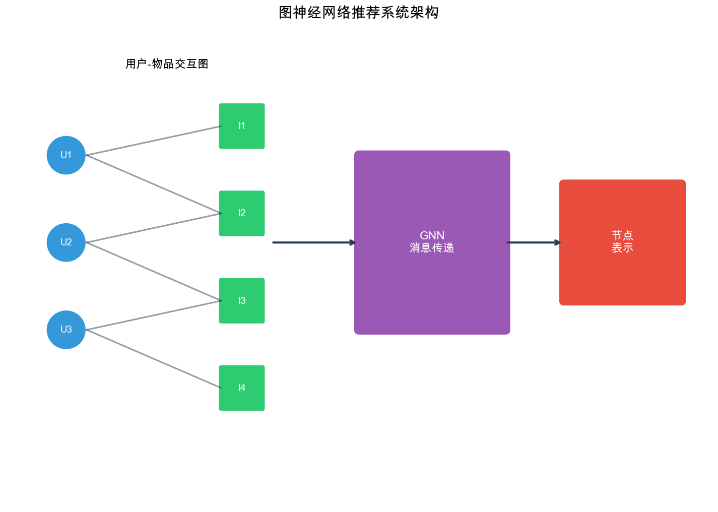
在推荐系统中,用户和物品之间的关系天然地构成了一个图结构:用户与物品之间的交互形成边,用户与用户之间的社交关系也形成边,物品与物品之间的相似性同样可以建模为边。传统的协同过滤和矩阵分解方法虽然有效,但它们往往将这种图结构信息"扁平化"处理,丢失了丰富的结构信息。
图神经网络( Graph Neural Networks,
GNN)的出现,为推荐系统带来了新的可能性。 GNN
能够直接在图上进行信息传播和聚合,捕捉用户和物品之间的高阶关系,从而学习到更丰富的表示。从
Pinterest 的 PinSage 到阿里巴巴的 LightGCN,从神经图协同过滤 NGCF
到社交推荐系统, GNN 在推荐领域展现出了强大的能力。
本文将深入探讨图神经网络在推荐系统中的应用,从 GNN 的基础原理( GCN
、 GAT 、
GraphSAGE)开始,逐步深入到推荐场景中的图建模、经典模型实现、社交推荐,以及图采样和训练技巧。我们会提供完整的代码实现,帮助读者从理论到实践全面掌握这一技术。
图神经网络基础
图的基本概念
在深入 GNN 之前,需要先理解图的基本概念。
什么是图( Graph)?
直觉理解:
图是一种描述"关系网络"的数据结构。它由两部分组成:
节点( Node/Vertex) :网络中的实体
例如:社交网络中的人、推荐系统中的用户/物品、知识图谱中的概念
边( Edge) :节点之间的关系或连接
例如:社交网络中的好友关系、推荐系统中的点击/购买行为、知识图谱中的"属于"关系
生活中的例子:
社交网络 :微信好友关系
地图导航 :城市交通网络
推荐系统 :用户-物品交互
节点 = 用户 + 物品
边 = 点击/购买/评分
形式化表示
图
-
符号说明:
-
在推荐系统中,常见的图结构包括:
用户-物品二部图( Bipartite Graph) :
节点 :用户节点边 :用户与物品之间的交互(点击、购买、评分等)
例如: Alice 点击了电影 A, Bob 购买了电影 B
特点 :用户节点之间没有直接连接,物品节点之间也没有直接连接
这叫"二部图":节点分为两组,边只连接不同组的节点
为什么是二部图?
在推荐场景中:
用户不会直接"连接"另一个用户(虽然可能有社交关系,但那是另一个图)
物品不会直接"连接"另一个物品(虽然可能相似,但边表示的是交互)
边总是"用户→物品"或"物品→用户"
社交图( Social Graph) :
节点 :用户边 :用户之间的关注、好友关系特点 :通常是无向图(双向好友)或有向图(单向关注)
知识图谱( Knowledge Graph) :
节点 :实体(用户、物品、属性等)边 :实体之间的关系(如"喜欢"、"属于"、"相似"等)特点 :包含多种类型的节点和边(异构图)
邻接矩阵( Adjacency Matrix) :图Extra close brace or missing open brace A \in \{0,1} ^{n \times n} ( 有 边 连 接 ) ( 无 边 连 接 )
直觉理解:
邻接矩阵是一个
行
值为 0 表示无连接
例子: 假设有 4 个节点,边集合为
性质:
对于无向图,
对于有向图,
对角线通常为 0(节点不连接自己),但添加自连接时可以为 1
度( Degree) :节点
直觉: 度表示节点的"连接数"或"流行度"
社交网络中:度高的用户有很多好友(社交达人)
推荐系统中:度高的物品被很多用户交互过(热门物品)
度矩阵( Degree Matrix) :对角矩阵
作用:
度矩阵用于归一化邻接矩阵,防止度大的节点主导信息传播。
图神经网络的核心思想
图神经网络的核心思想是消息传递( Message
Passing) :每个节点通过聚合邻居节点的信息来更新自己的表示。
直觉:社交网络中的信息传播
想象你在社交网络上:
初始状态 :每个人有自己的兴趣(节点特征)
Alice 喜欢电影
Bob 喜欢音乐
Carol 喜欢运动
消息传递 :你会受到好友的影响
Alice 看到 Bob 在听音乐,开始对音乐感兴趣
Bob 看到 Carol 在运动,也想尝试运动
经过多次交流,大家的兴趣逐渐融合
更新表示 :每个人的兴趣变成了自己+好友兴趣的混合
Alice 现在喜欢:电影(主要)+ 音乐(来自 Bob)
Bob 现在喜欢:音乐(主要)+ 电影(来自 Alice)+ 运动(来自
Carol)
这就是 GNN
的核心:通过邻居的信息丰富自己的表示 。
为什么这样有用?
在推荐系统中:
用户节点 :如果两个用户交互过相似的物品(有共同邻居),他们可能有相似的偏好物品节点 :如果两个物品被相似的用户喜欢(有共同邻居),它们可能相似
通过消息传递, GNN 可以捕捉这种高阶相似性 :
1 阶 :用户直接交互的物品(协同过滤已经能做)2 阶 :交互过相似物品的其他用户喜欢的物品("买了 A
的人也买了 B")3 阶及更高 :更复杂的关联模式
形式化定义
GNN 的每一层执行以下操作:
消息生成(
Message) :每个节点生成发送给邻居的消息消息聚合(
Aggregate) :每个节点聚合来自邻居的消息节点更新(
Update) :根据聚合的消息更新节点表示
对于节点Extra close brace or missing open brace \mathbf{h}_v^{(l+1)} = \text{UPDATE}^{(l)}\left(\mathbf{h}_v^{(l)}, \text{AGGREGATE}^{(l)}\left(\{\mathbf{h}_u^{(l)} : u \in \mathcal{N}(v)} \right)\right)
符号说明:
-
直觉理解(推荐场景):
假设我们要更新用户 Alice 的表示:
第 0 层 :初始嵌入(随机初始化或从 ID 学习)
第 1 层 :聚合 Alice 交互过的物品的信息
邻居:电影 A 、电影 B 、电影 C
聚合:邻 居 聚 合 含义 : Alice
的表示现在包含了她喜欢的电影的信息
第 2
层 :再次聚合,这次邻居的表示已经包含了它们的邻居信息
电影 A 的表示
Alice 的 2 层表示包含了"喜欢相似电影的其他用户"的信息
含义 :捕捉到了 2 阶相似性
为什么多层有用?
1 层 :直接邻居(用户喜欢的物品)2
层 :邻居的邻居(喜欢相似物品的用户喜欢的其他物品)3 层 :更高阶的关联模式
但也不是越多越好:
过多层 :导致过平滑 (所有节点表示变得相似),丧失个性化通常 : 2-3 层就足够了
图卷积网络( GCN)
图卷积网络( Graph Convolutional Network, GCN)是 GNN
的经典模型之一,由 Kipf & Welling 在 2017 年提出。
为什么需要 GCN?(动机)
传统神经网络( CNN 、
RNN)处理的是规则结构数据 :
CNN:图像(规则的 2D 网格)
RNN:序列(有固定的前后关系)
但图数据是不规则 的:
每个节点的邻居数量不同(有的用户交互了 10 个物品,有的交互了 1000
个)
没有固定的顺序(邻居没有"第一个"、"第二个"的概念)
GCN 的目标:设计一种在图上做"卷积"的操作,能够:
聚合邻居信息(类似 CNN 的感受野)
处理任意数量的邻居
对邻居顺序不敏感(置换不变性)
GCN 的数学形式 :
GCN 使用对称归一化的邻接矩阵进行信息传播:
符号说明:
-作用 :让每个节点在聚合时也包含自己的信息
-
-
-$^{(l)} ^{d_l d_{l+1}} : 可 学 习 的 权 重 矩 阵 将 维 特 征 映 射 到
-
归一化的作用:
问题 1:不归一化会怎样?
如果直接用
度大的节点(邻居多)会获得更大的数值
例如:节点 A 有 100 个邻居,节点 B 有 5 个邻居
A 聚合后的值是 B 的 20 倍!
随着层数增加,数值会爆炸或消失
训练不稳定
问题 2:为什么是
对称归一化$^{-} ^{-} 的 每 个 元 素 为 :
直觉理解:
当节点
度大的节点接收和发送的信息都会被"削弱"
保证聚合后的数值范围稳定
为什么这样设计有效?
数值稳定 :权重矩阵的特征值被限制在合理范围信息均衡 :度大的节点不会主导信息传播理论保证 :对应于图拉普拉斯矩阵的谱分解(与信号处理中的傅里叶变换类似)
节点级别的表示 :
对于单个节点Extra close brace or missing open brace \mathbf{h}_v^{(l+1)} = \sigma\left(\sum_{u \in \mathcal{N}(v) \cup \{v} } \frac{1}{\sqrt{d_v d_u}} \mathbf{h}_u^{(l)} \mathbf{W}^{(l)}\right)
直觉理解(逐步拆解):
Extra close brace or missing open brace \sum_{u \in \mathcal{N}(v) \cup \{v} }
权重反比于度的平方根乘积
完整流程示例:
假设用户 Alice(度=3)的邻居是电影 A(度=100)、电影 B(度=50):
邻居权重:
自己:加 权 聚 合 : {} ^{} = 0.33 {} +
0.058 _A + 0.082 _B特 征 变 换 : 乘 以 权 重 矩 阵
关键洞察:
热门物品(度大)不会因为被很多用户喜欢而过度影响单个用户的表示。每个邻居的贡献被归一化了。
GCN 实现 :
1
2
3
4
5
6
7
8
9
10
11
12
13
14
15
16
17
18
19
20
21
22
23
24
25
26
27
28
29
30
31
32
33
34
35
36
37
38
39
40
41
42
43
44
45
46
47
48
49
50
51
52
53
54
55
56
57
58
59
60
61
62
63
64
65
66
67
68
69
70
import torchimport torch.nn as nnimport torch.nn.functional as Ffrom torch_geometric.nn import MessagePassingfrom torch_geometric.utils import add_self_loops, degreeclass GCNLayer (nn.Module): """GCN 单层实现""" def __init__ (self, in_channels, out_channels ): super (GCNLayer, self).__init__() self.linear = nn.Linear(in_channels, out_channels) self.reset_parameters() def reset_parameters (self ): nn.init.xavier_uniform_(self.linear.weight) nn.init.zeros_(self.linear.bias) def forward (self, x, edge_index ): """ Args: x: 节点特征矩阵 [num_nodes, in_channels] edge_index: 边索引 [2, num_edges] Returns: 更新后的节点特征 [num_nodes, out_channels] """ edge_index, _ = add_self_loops(edge_index, num_nodes=x.size(0 )) row, col = edge_index deg = degree(col, x.size(0 ), dtype=x.dtype) deg_inv_sqrt = deg.pow (-0.5 ) deg_inv_sqrt[deg_inv_sqrt == float ('inf' )] = 0 norm = deg_inv_sqrt[row] * deg_inv_sqrt[col] x = self.linear(x) x = self.propagate(edge_index, x=x, norm=norm) return x def message (self, x_j, norm ): """消息函数:计算发送的消息""" return norm.view(-1 , 1 ) * x_j class GCN (nn.Module): """多层 GCN 模型""" def __init__ (self, num_nodes, in_channels, hidden_channels, out_channels, num_layers=2 , dropout=0.5 ): super (GCN, self).__init__() self.num_layers = num_layers self.dropout = dropout self.layers = nn.ModuleList() self.layers.append(GCNLayer(in_channels, hidden_channels)) for _ in range (num_layers - 2 ): self.layers.append(GCNLayer(hidden_channels, hidden_channels)) if num_layers > 1 : self.layers.append(GCNLayer(hidden_channels, out_channels)) def forward (self, x, edge_index ): for i, layer in enumerate (self.layers): x = layer(x, edge_index) if i < len (self.layers) - 1 : x = F.relu(x) x = F.dropout(x, p=self.dropout, training=self.training) return x
图注意力网络( GAT)
图注意力网络( Graph Attention Network,
GAT)引入了注意力机制,允许节点自适应地选择重要的邻居进行信息聚合。
GAT 的核心思想 :
GAT 为每条边
注意力机制 :
对于节点
其中: -
然后使用 softmax 归一化得到注意力权重:
节点更新 :
节点
多头注意力 :
GAT 通常使用多头注意力( Multi-head
Attention)来稳定训练并捕捉不同类型的邻居关系:
其中
GAT 实现 :
1
2
3
4
5
6
7
8
9
10
11
12
13
14
15
16
17
18
19
20
21
22
23
24
25
26
27
28
29
30
31
32
33
34
35
36
37
38
39
40
41
42
43
44
45
46
47
48
49
50
51
52
53
54
55
56
57
58
59
60
61
62
63
64
65
66
67
68
69
70
71
72
73
74
75
76
77
78
79
80
81
82
83
84
85
86
87
88
89
90
91
92
93
94
95
96
97
import torchimport torch.nn as nnimport torch.nn.functional as Ffrom torch_geometric.nn import MessagePassingfrom torch_geometric.utils import add_self_loopsclass GATLayer (nn.Module): """GAT 单层实现""" def __init__ (self, in_channels, out_channels, heads=1 , dropout=0.6 , concat=True ): super (GATLayer, self).__init__() self.in_channels = in_channels self.out_channels = out_channels self.heads = heads self.concat = concat self.dropout = dropout self.W = nn.Parameter(torch.empty(size=(in_channels, out_channels * heads))) nn.init.xavier_uniform_(self.W.data, gain=1.414 ) self.a = nn.Parameter(torch.empty(size=(2 * out_channels, 1 ))) nn.init.xavier_uniform_(self.a.data, gain=1.414 ) self.leaky_relu = nn.LeakyReLU(0.2 ) def forward (self, x, edge_index ): """ Args: x: 节点特征 [num_nodes, in_channels] edge_index: 边索引 [2, num_edges] """ h = torch.mm(x, self.W) h = h.view(-1 , self.heads, self.out_channels) edge_index, _ = add_self_loops(edge_index, num_nodes=x.size(0 )) h_prime = self.propagate(edge_index, x=h) if self.concat: return h_prime.view(-1 , self.heads * self.out_channels) else : return h_prime.mean(dim=1 ) def message (self, x_i, x_j, edge_index_i ): """消息函数:计算注意力权重和消息""" x_cat = torch.cat([x_i, x_j], dim=-1 ) e = self.leaky_relu(torch.matmul(x_cat, self.a)) e = e.squeeze(-1 ) alpha = F.softmax(e, dim=0 ) alpha = F.dropout(alpha, p=self.dropout, training=self.training) return alpha.unsqueeze(-1 ) * x_j def aggregate (self, inputs, index, dim_size=None ): """聚合函数:对邻居消息求和""" return torch.scatter_add(inputs, index, dim=0 , dim_size=dim_size) class GAT (nn.Module): """多层 GAT 模型""" def __init__ (self, num_nodes, in_channels, hidden_channels, out_channels, num_layers=2 , heads=8 , dropout=0.6 ): super (GAT, self).__init__() self.num_layers = num_layers self.dropout = dropout self.layers = nn.ModuleList() self.layers.append(GATLayer(in_channels, hidden_channels, heads=heads, dropout=dropout, concat=True )) for _ in range (num_layers - 2 ): self.layers.append(GATLayer(hidden_channels * heads, hidden_channels, heads=heads, dropout=dropout, concat=True )) if num_layers > 1 : self.layers.append(GATLayer(hidden_channels * heads, out_channels, heads=heads, dropout=dropout, concat=False )) def forward (self, x, edge_index ): for i, layer in enumerate (self.layers): x = layer(x, edge_index) if i < len (self.layers) - 1 : x = F.elu(x) x = F.dropout(x, p=self.dropout, training=self.training) return x
GraphSAGE
GraphSAGE( Graph Sample and Aggregate)是一种归纳式( Inductive)的
GNN 模型,能够为未见过的节点生成嵌入。
GraphSAGE 的核心思想 :
与 GCN 不同, GraphSAGE
不要求所有节点在训练时都存在,它通过采样和聚合邻居来学习节点的表示。
采样策略 :
GraphSAGE 使用固定大小的邻居采样: - 对于每个节点,随机采样
聚合函数 :
GraphSAGE 支持多种聚合函数:
平均聚合(Mean Aggregator) :
LSTM 聚合 :使用 LSTM
处理邻居序列(需要固定顺序)
池化聚合(Pooling Aggregator) :Extra close brace or missing open brace \mathbf{h}_v^{(l+1)} = \sigma\left(\mathbf{W}^{(l)} \cdot \text{CONCAT}\left(\mathbf{h}_v^{(l)}, \text{MAX}\left(\{\sigma(\mathbf{W}_{pool}\mathbf{h}_u^{(l)} + \mathbf{b}) : u \in \mathcal{N}(v)} \right)\right)\right)
GraphSAGE 实现 :
1
2
3
4
5
6
7
8
9
10
11
12
13
14
15
16
17
18
19
20
21
22
23
24
25
26
27
28
29
30
31
32
33
34
35
36
37
38
39
40
41
42
43
44
45
46
47
48
49
50
51
52
53
54
55
56
57
58
59
60
import torchimport torch.nn as nnimport torch.nn.functional as Ffrom torch_geometric.nn import SAGEConvfrom torch_geometric.data import Data, NeighborSamplerclass GraphSAGE (nn.Module): """GraphSAGE 模型实现""" def __init__ (self, in_channels, hidden_channels, out_channels, num_layers=2 , dropout=0.5 ): super (GraphSAGE, self).__init__() self.num_layers = num_layers self.dropout = dropout self.convs = nn.ModuleList() self.convs.append(SAGEConv(in_channels, hidden_channels)) for _ in range (num_layers - 2 ): self.convs.append(SAGEConv(hidden_channels, hidden_channels)) if num_layers > 1 : self.convs.append(SAGEConv(hidden_channels, out_channels)) def forward (self, x, edge_index ): for i, conv in enumerate (self.convs): x = conv(x, edge_index) if i < len (self.convs) - 1 : x = F.relu(x) x = F.dropout(x, p=self.dropout, training=self.training) return x def train_graphsage_with_sampling (model, data, train_loader, optimizer, device ): """使用邻居采样训练 GraphSAGE""" model.train() total_loss = 0 for batch_size, n_id, adjs in train_loader: optimizer.zero_grad() x = data.x[n_id].to(device) for i, (edge_index, _, size) in enumerate (adjs): edge_index = edge_index.to(device) x = model.convs[i](x, edge_index) if i < len (adjs) - 1 : x = F.relu(x) x = F.dropout(x, p=model.dropout, training=model.training) return total_loss / len (train_loader)
推荐系统中的图建模
用户-物品二部图
推荐系统中最基本的图结构是用户-物品二部图( User-Item Bipartite
Graph)。
图定义 :
节点集合 :边集合 :Extra close brace or missing open brace E = \{(u, i) : u \in U, i \in I, \text{用户 } u \text{ 与物品 } i \text{ 有交互}} 边权重 :可以是评分、点击次数、购买次数等
邻接矩阵 :
用户-物品二部图的邻接矩阵可以表示为:
其中
二部图的特点 :
无三角形结构 :用户节点之间没有直接连接,物品节点之间也没有直接连接高阶关系 :用户可以通过共同喜欢的物品建立间接关系,物品可以通过被相同用户喜欢建立间接关系信息传播 : GNN
可以在二部图上进行信息传播,学习用户和物品的表示
异构图建模
除了简单的二部图,推荐系统还可以构建更复杂的异构图( Heterogeneous
Graph)。
节点类型 : - 用户节点 - 物品节点 -
属性节点(类别、标签、品牌等) - 上下文节点(时间、地点等)
边类型 : - 用户-物品交互边(点击、购买、评分等) -
用户-用户社交边(关注、好友) - 物品-属性边(属于、包含) -
用户-属性边(偏好)
异构图示例 :
1
2
3
用户 1 --[点击]--> 物品 A --[属于]--> 类别 1 用户 1 --[关注]--> 用户 2 --[购买]--> 物品 B 物品 A --[相似]--> 物品 C
图构建策略
基于交互的边 : - 显式反馈:评分、评论 -
隐式反馈:点击、浏览、购买、收藏
边权重设计 : - 二值权重:有交互为 1,无交互为 0 -
频率权重:交互次数 - 时间衰减权重:
负采样边 : -
对于隐式反馈,需要采样负样本(用户未交互的物品) -
常用策略:随机负采样、基于流行度的负采样
PinSage: Pinterest
的大规模图推荐系统
PinSage 是 Pinterest 在 2018
年提出的用于大规模推荐系统的图神经网络模型,它能够处理包含 30 亿节点和
180 亿边的超大规模图。
PinSage 的核心设计
主要创新点 :
重要性采样( Importance-based
Sampling) :不是随机采样邻居,而是根据重要性采样卷积聚合 :使用可学习的聚合函数随机游走重要性 :使用随机游走计算节点重要性高效训练 :支持大规模图的训练和推理
重要性采样
PinSage 使用随机游走计算节点的重要性分数:
对于节点
然后根据重要性分数采样 Top-K 邻居:
PinSage 聚合函数
PinSage 使用卷积聚合( Convolve)来聚合邻居信息:Extra close brace or missing open brace \mathbf{h}_v^{(l+1)} = \sigma\left(\mathbf{W}^{(l)} \cdot \text{CONCAT}\left[\mathbf{h}_v^{(l)}, \text{AGGREGATE}\left(\{\mathbf{h}_u^{(l)} : u \in \mathcal{N}(v)} \right)\right]\right)
其中 AGGREGATE 函数可以是: - 加权平均:根据重要性分数加权 -
最大池化:取最大值 - LSTM:使用 LSTM 处理邻居序列
PinSage 实现
1
2
3
4
5
6
7
8
9
10
11
12
13
14
15
16
17
18
19
20
21
22
23
24
25
26
27
28
29
30
31
32
33
34
35
36
37
38
39
40
41
42
43
44
45
46
47
48
49
50
51
52
53
54
55
56
57
58
59
60
61
62
63
64
65
66
67
68
69
70
71
72
73
74
75
76
77
78
79
80
81
82
83
84
85
86
87
88
89
90
91
92
93
94
95
96
97
98
99
100
101
102
103
104
105
106
107
108
109
110
111
112
113
114
115
116
117
118
119
import torchimport torch.nn as nnimport torch.nn.functional as Fimport numpy as npfrom collections import defaultdictclass PinSageLayer (nn.Module): """PinSage 单层实现""" def __init__ (self, in_channels, out_channels, num_samples=25 , aggregator='mean' ): super (PinSageLayer, self).__init__() self.in_channels = in_channels self.out_channels = out_channels self.num_samples = num_samples self.aggregator = aggregator self.conv = nn.Linear(in_channels * 2 , out_channels) if aggregator == 'lstm' : self.lstm = nn.LSTM(in_channels, in_channels, batch_first=True ) def forward (self, node_features, neighbors_list, importance_scores=None ): """ Args: node_features: 节点特征字典 {node_id: feature_vector} neighbors_list: 每个节点的邻居列表 {node_id: [neighbor_ids]} importance_scores: 重要性分数 {node_id: {neighbor_id: score }} """ aggregated_features = {} for node_id, neighbors in neighbors_list.items(): if len (neighbors) == 0 : aggregated_features[node_id] = node_features[node_id] continue if len (neighbors) > self.num_samples: if importance_scores and node_id in importance_scores: neighbor_scores = [(n, importance_scores[node_id].get(n, 0 )) for n in neighbors] neighbor_scores.sort(key=lambda x: x[1 ], reverse=True ) sampled_neighbors = [n for n, _ in neighbor_scores[:self.num_samples]] else : sampled_neighbors = np.random.choice(neighbors, self.num_samples, replace=False ).tolist() else : sampled_neighbors = neighbors neighbor_features = [node_features[n] for n in sampled_neighbors] neighbor_features = torch.stack(neighbor_features) if self.aggregator == 'mean' : aggregated = neighbor_features.mean(dim=0 ) elif self.aggregator == 'max' : aggregated = neighbor_features.max (dim=0 )[0 ] elif self.aggregator == 'lstm' : aggregated, _ = self.lstm(neighbor_features.unsqueeze(0 )) aggregated = aggregated[0 , -1 ] else : raise ValueError(f"Unknown aggregator: {self.aggregator} " ) combined = torch.cat([node_features[node_id], aggregated], dim=-1 ) aggregated_features[node_id] = self.conv(combined) return aggregated_features class PinSage (nn.Module): """PinSage 模型""" def __init__ (self, num_nodes, in_channels, hidden_channels, out_channels, num_layers=2 , num_samples=25 , aggregator='mean' ): super (PinSage, self).__init__() self.num_layers = num_layers self.layers = nn.ModuleList() self.layers.append(PinSageLayer(in_channels, hidden_channels, num_samples, aggregator)) for _ in range (num_layers - 2 ): self.layers.append(PinSageLayer(hidden_channels, hidden_channels, num_samples, aggregator)) if num_layers > 1 : self.layers.append(PinSageLayer(hidden_channels, out_channels, num_samples, aggregator)) def forward (self, node_features, neighbors_list, importance_scores=None ): x = node_features for layer in self.layers: x = layer(x, neighbors_list, importance_scores) x = {k: F.relu(v) for k, v in x.items()} return x def compute_random_walk_importance (graph, root_node, num_walks=100 , walk_length=5 ): """计算随机游走重要性分数""" importance = defaultdict(float ) for _ in range (num_walks): current = root_node for step in range (walk_length): if current not in graph: break neighbors = graph[current] if len (neighbors) == 0 : break current = np.random.choice(neighbors) importance[current] += 1.0 / (step + 1 ) return importance
PinSage 训练技巧
负采样 : - 对于每个正样本硬负样本挖掘 : -
不仅随机采样负样本,还采样"困难"的负样本(与用户历史交互物品相似的未交互物品)
- 提高模型的区分能力
批量训练 : - 使用 mini-batch 训练,每个 batch
包含多个用户及其邻居子图 - 使用图采样技术减少计算量
LightGCN:简化的图卷积推荐
LightGCN 是 2020 年提出的简化版图卷积推荐模型,它去除了 GCN
中的特征变换和非线性激活,只保留最核心的邻域聚合操作。
LightGCN 的设计理念
传统 GCN 的问题 : -
特征变换(线性层)可能不适合推荐任务 -
非线性激活可能增加模型复杂度,但收益有限 - 自连接可能引入噪声
LightGCN 的简化 : - 移除特征变换和非线性激活 -
移除自连接 - 只保留邻域聚合
LightGCN 的数学形式
LightGCN 的层更新公式:
其中: -
最终嵌入 :
LightGCN 将各层的嵌入加权求和作为最终嵌入:
其中
预测分数 :
用户
LightGCN 实现
问题背景
传统的图神经网络方法(如 GCN 、
NGCF)在推荐系统中虽然有效,但存在一些问题:(
1)模型复杂度高,包含特征变换、非线性激活等操作,训练和推理速度较慢;(
2)对于推荐任务,这些复杂的操作可能不是必需的,甚至可能引入噪声;(
3)在用户-物品二部图中,用户和物品的特征往往是 ID
嵌入,特征变换的作用有限。如何设计一个简单高效的 GNN
模型,既能捕获图结构信息,又能保持训练和推理的高效性,是推荐系统中的一个重要挑战。
解决思路
LightGCN( Light Graph Convolutional
Network)是专门为推荐系统设计的简化版 GCN 。基本思路:移除 GCN
中的特征变换和非线性激活,只保留最核心的邻域聚合操作。 LightGCN
认为,对于推荐任务,图结构信息比特征变换更重要,简单的邻域聚合就足以学习有效的节点表示。具体而言,
LightGCN
的每一层只进行邻域聚合,然后将所有层的表示进行加权求和得到最终表示。这种设计大幅简化了模型,提升了训练和推理速度,同时在推荐任务上取得了更好的效果。
设计考虑
在实现 LightGCN 时,需要考虑以下几个关键设计:
简化的图卷积 : LightGCN
移除了特征变换和非线性激活,每一层只进行邻域聚合。对于用户-物品二部图,用户节点的表示通过聚合其交互的物品节点得到,物品节点的表示通过聚合其交互的用户节点得到。这种设计使得模型更加轻量,训练和推理速度更快。
层组合策略 : LightGCN
将所有层的表示进行加权求和得到最终表示,而不是只使用最后一层。这种设计能够同时利用不同层的信息:浅层捕获局部结构,深层捕获全局结构。通常使用均匀权重或可学习的权重,实验表明均匀权重效果已经很好。
嵌入初始化 : LightGCN
使用随机初始化的嵌入,不需要预训练。嵌入维度通常设置为 64-256
维,根据用户和物品数量选择。
训练策略 : LightGCN 使用 BPR
损失进行训练,最大化正样本(用户-物品交互)的得分,最小化负样本的得分。训练时使用负采样策略,每个正样本对应多个负样本。
1
2
3
4
5
6
7
8
9
10
11
12
13
14
15
16
17
18
19
20
21
22
23
24
25
26
27
28
29
30
31
32
33
34
35
36
37
38
39
40
41
42
43
44
45
46
47
48
49
50
51
52
53
54
55
56
57
58
59
60
61
62
63
64
65
66
67
68
69
70
71
72
73
74
75
76
77
78
79
80
81
82
83
84
85
86
87
88
89
90
91
92
93
94
95
96
97
98
99
100
101
102
103
104
105
106
107
108
109
110
111
112
113
114
115
116
117
118
119
120
121
122
123
124
125
126
127
128
129
130
131
132
133
134
135
136
137
138
139
140
141
142
143
144
145
146
147
148
149
150
151
152
153
154
155
156
157
158
159
160
161
162
163
164
165
166
167
import torchimport torch.nn as nnimport torch.nn.functional as Fimport numpy as npfrom scipy.sparse import coo_matrixclass LightGCN (nn.Module): """LightGCN 模型实现""" def __init__ (self, num_users, num_items, embedding_dim=64 , num_layers=3 ): super (LightGCN, self).__init__() self.num_users = num_users self.num_items = num_items self.embedding_dim = embedding_dim self.num_layers = num_layers self.user_embedding = nn.Embedding(num_users, embedding_dim) self.item_embedding = nn.Embedding(num_items, embedding_dim) nn.init.normal_(self.user_embedding.weight, std=0.1 ) nn.init.normal_(self.item_embedding.weight, std=0.1 ) self.alpha = 1.0 / (num_layers + 1 ) def forward (self, user_indices, item_indices, graph ): """ Args: user_indices: 用户索引 [batch_size] item_indices: 物品索引 [batch_size] graph: 图结构(邻接矩阵或边索引) Returns: 用户和物品的嵌入 """ user_emb = self.user_embedding.weight item_emb = self.item_embedding.weight user_embeddings = [user_emb] item_embeddings = [item_emb] for _ in range (self.num_layers): user_emb = self._propagate_users(user_emb, item_embeddings[-1 ], graph) user_embeddings.append(user_emb) item_emb = self._propagate_items(item_emb, user_embeddings[-2 ], graph) item_embeddings.append(item_emb) final_user_emb = sum ([self.alpha * emb for emb in user_embeddings]) final_item_emb = sum ([self.alpha * emb for emb in item_embeddings]) user_emb_batch = final_user_emb[user_indices] item_emb_batch = final_item_emb[item_indices] return user_emb_batch, item_emb_batch def _propagate_users (self, user_emb, item_emb, graph ): """用户嵌入传播:聚合邻居物品""" return user_emb def _propagate_items (self, item_emb, user_emb, graph ): """物品嵌入传播:聚合邻居用户""" return item_emb def predict (self, user_indices, item_indices, graph ): """预测用户对物品的评分""" user_emb, item_emb = self.forward(user_indices, item_indices, graph) scores = (user_emb * item_emb).sum (dim=1 ) return scores class LightGCNWithSparseGraph (nn.Module): """使用稀疏矩阵的 LightGCN 实现""" def __init__ (self, num_users, num_items, embedding_dim=64 , num_layers=3 ): super (LightGCNWithSparseGraph, self).__init__() self.num_users = num_users self.num_items = num_items self.embedding_dim = embedding_dim self.num_layers = num_layers self.user_embedding = nn.Embedding(num_users, embedding_dim) self.item_embedding = nn.Embedding(num_items, embedding_dim) nn.init.normal_(self.user_embedding.weight, std=0.1 ) nn.init.normal_(self.item_embedding.weight, std=0.1 ) self.alpha = 1.0 / (num_layers + 1 ) def build_graph (self, user_item_pairs ): """构建归一化的图结构""" users, items = zip (*user_item_pairs) users = np.array(users) items = np.array(items) num_nodes = self.num_users + self.num_items user_degrees = np.bincount(users, minlength=self.num_users) item_degrees = np.bincount(items, minlength=self.num_items) row = np.concatenate([users, items + self.num_users]) col = np.concatenate([items + self.num_users, users]) norm = np.concatenate([ 1.0 / np.sqrt(user_degrees[users] * item_degrees[items]), 1.0 / np.sqrt(user_degrees[users] * item_degrees[items]) ]) from scipy.sparse import coo_matrix adj_matrix = coo_matrix((norm, (row, col)), shape=(num_nodes, num_nodes)) return adj_matrix def forward (self, user_indices, item_indices, adj_matrix ): """前向传播""" all_embeddings = torch.cat([ self.user_embedding.weight, self.item_embedding.weight ], dim=0 ) embeddings_list = [all_embeddings] adj_tensor = self._sparse_matrix_to_tensor(adj_matrix).to(all_embeddings.device) for _ in range (self.num_layers): all_embeddings = torch.sparse.mm(adj_tensor, all_embeddings) embeddings_list.append(all_embeddings) final_embeddings = sum ([self.alpha * emb for emb in embeddings_list]) user_emb = final_embeddings[:self.num_users] item_emb = final_embeddings[self.num_users:] return user_emb[user_indices], item_emb[item_indices] def _sparse_matrix_to_tensor (self, sparse_matrix ): """将 scipy 稀疏矩阵转换为 PyTorch 稀疏张量""" values = sparse_matrix.data indices = np.vstack((sparse_matrix.row, sparse_matrix.col)) i = torch.LongTensor(indices) v = torch.FloatTensor(values) shape = sparse_matrix.shape return torch.sparse.FloatTensor(i, v, torch.Size(shape))
NGCF:神经图协同过滤
NGCF( Neural Graph Collaborative Filtering)是 2019 年提出的将 GCN
应用于协同过滤的模型。
NGCF 的核心思想
NGCF 将用户-物品交互建模为二部图,使用 GCN
在图上进行信息传播,学习用户和物品的嵌入表示。
与传统矩阵分解的区别 : - 矩阵分解只考虑直接交互 -
NGCF 通过多层 GCN 捕捉高阶交互关系
NGCF 的数学形式
NGCF 的嵌入传播规则:
第一层传播 :
第 :
其中: -
最终嵌入 :
将各层嵌入拼接:
预测分数 :
NGCF 实现
1
2
3
4
5
6
7
8
9
10
11
12
13
14
15
16
17
18
19
20
21
22
23
24
25
26
27
28
29
30
31
32
33
34
35
36
37
38
39
40
41
42
43
44
45
46
47
48
49
50
51
52
53
54
55
56
57
58
59
60
61
62
63
64
65
66
67
68
69
70
71
72
73
74
75
76
77
78
79
80
81
82
83
84
85
86
87
88
89
90
91
92
93
94
95
96
97
98
99
100
101
102
103
104
105
106
107
108
109
110
111
112
113
114
115
116
117
118
119
120
121
122
123
124
125
126
127
128
129
130
131
132
133
134
135
136
137
138
139
140
141
142
143
144
145
146
147
148
149
150
import torchimport torch.nn as nnimport torch.nn.functional as Fimport numpy as npfrom scipy.sparse import coo_matrixclass NGCFLayer (nn.Module): """NGCF 单层实现""" def __init__ (self, in_dim, out_dim, dropout=0.0 ): super (NGCFLayer, self).__init__() self.in_dim = in_dim self.out_dim = out_dim self.dropout = dropout self.W1 = nn.Linear(in_dim, out_dim, bias=False ) self.W2 = nn.Linear(in_dim, out_dim, bias=False ) self.reset_parameters() def reset_parameters (self ): nn.init.xavier_uniform_(self.W1.weight) nn.init.xavier_uniform_(self.W2.weight) def forward (self, user_emb, item_emb, user_item_graph, item_user_graph ): """ Args: user_emb: 用户嵌入 [num_users, in_dim] item_emb: 物品嵌入 [num_items, in_dim] user_item_graph: 用户-物品图(稀疏矩阵) item_user_graph: 物品-用户图(稀疏矩阵) """ user_emb_self = self.W1(user_emb) item_to_user = torch.sparse.mm(user_item_graph, item_emb) item_to_user = self.W1(item_to_user) user_item_interaction = torch.sparse.mm(user_item_graph, item_emb * user_emb) user_item_interaction = self.W2(user_item_interaction) user_emb_new = user_emb_self + item_to_user + user_item_interaction user_emb_new = F.leaky_relu(user_emb_new, negative_slope=0.2 ) user_emb_new = F.dropout(user_emb_new, p=self.dropout, training=self.training) item_emb_self = self.W1(item_emb) user_to_item = torch.sparse.mm(item_user_graph, user_emb) user_to_item = self.W1(user_to_item) item_user_interaction = torch.sparse.mm(item_user_graph, user_emb * item_emb) item_user_interaction = self.W2(item_user_interaction) item_emb_new = item_emb_self + user_to_item + item_user_interaction item_emb_new = F.leaky_relu(item_emb_new, negative_slope=0.2 ) item_emb_new = F.dropout(item_emb_new, p=self.dropout, training=self.training) return user_emb_new, item_emb_new class NGCF (nn.Module): """NGCF 模型""" def __init__ (self, num_users, num_items, embedding_dim=64 , num_layers=3 , dropout=0.1 ): super (NGCF, self).__init__() self.num_users = num_users self.num_items = num_items self.embedding_dim = embedding_dim self.num_layers = num_layers self.user_embedding = nn.Embedding(num_users, embedding_dim) self.item_embedding = nn.Embedding(num_items, embedding_dim) nn.init.normal_(self.user_embedding.weight, std=0.1 ) nn.init.normal_(self.item_embedding.weight, std=0.1 ) self.layers = nn.ModuleList() for i in range (num_layers): self.layers.append(NGCFLayer(embedding_dim, embedding_dim, dropout)) def build_graph (self, user_item_pairs ): """构建图结构""" users, items = zip (*user_item_pairs) users = np.array(users) items = np.array(items) user_degrees = np.bincount(users, minlength=self.num_users) item_degrees = np.bincount(items, minlength=self.num_items) norm_user_item = 1.0 / np.sqrt(user_degrees[users] * item_degrees[items]) user_item_graph = coo_matrix( (norm_user_item, (users, items)), shape=(self.num_users, self.num_items) ) item_user_graph = user_item_graph.T return user_item_graph, item_user_graph def forward (self, user_indices, item_indices, user_item_graph, item_user_graph ): """前向传播""" user_emb = self.user_embedding.weight item_emb = self.item_embedding.weight user_embeddings = [user_emb] item_embeddings = [item_emb] user_item_tensor = self._sparse_matrix_to_tensor(user_item_graph).to(user_emb.device) item_user_tensor = self._sparse_matrix_to_tensor(item_user_graph).to(item_emb.device) for layer in self.layers: user_emb, item_emb = layer(user_emb, item_emb, user_item_tensor, item_user_tensor) user_embeddings.append(user_emb) item_embeddings.append(item_emb) final_user_emb = torch.cat(user_embeddings, dim=1 ) final_item_emb = torch.cat(item_embeddings, dim=1 ) return final_user_emb[user_indices], final_item_emb[item_indices] def predict (self, user_indices, item_indices, user_item_graph, item_user_graph ): """预测评分""" user_emb, item_emb = self.forward(user_indices, item_indices, user_item_graph, item_user_graph) scores = (user_emb * item_emb).sum (dim=1 ) return scores def _sparse_matrix_to_tensor (self, sparse_matrix ): """转换为 PyTorch 稀疏张量""" values = sparse_matrix.data indices = np.vstack((sparse_matrix.row, sparse_matrix.col)) i = torch.LongTensor(indices) v = torch.FloatTensor(values) shape = sparse_matrix.shape return torch.sparse.FloatTensor(i, v, torch.Size(shape))
社交推荐系统
社交推荐( Social
Recommendation)利用用户之间的社交关系来提升推荐效果。
社交推荐的基本思想
核心假设 : - 用户倾向于喜欢其社交好友喜欢的物品 -
社交关系可以提供额外的信号来缓解数据稀疏性问题 -
社交影响力会影响用户的决策
社交图的构建
社交关系类型 : - 显式关系:关注、好友、粉丝 -
隐式关系:共同兴趣、相似行为
社交图表示 : - 无向图:好友关系 - 有向图:关注关系 -
加权图:关系强度
社交推荐模型
SoRec( Social Recommendation) :
结合用户-物品交互和用户-用户社交关系:
其中
SocialMF : 使用矩阵分解同时建模交互和社交关系:
其中
GraphRec( Graph Neural Network for Social
Recommendation) : 使用 GNN
同时建模用户-物品交互和用户-用户社交关系。
GraphRec 实现
1
2
3
4
5
6
7
8
9
10
11
12
13
14
15
16
17
18
19
20
21
22
23
24
25
26
27
28
29
30
31
32
33
34
35
36
37
38
39
40
41
42
43
44
45
46
47
48
49
50
51
52
53
54
55
56
57
58
import torchimport torch.nn as nnimport torch.nn.functional as Fclass GraphRec (nn.Module): """GraphRec: 社交推荐模型""" def __init__ (self, num_users, num_items, embedding_dim=64 , social_graph=None , num_layers=2 ): super (GraphRec, self).__init__() self.num_users = num_users self.num_items = num_items self.embedding_dim = embedding_dim self.user_embedding = nn.Embedding(num_users, embedding_dim) self.item_embedding = nn.Embedding(num_items, embedding_dim) if social_graph is not None : self.social_embedding = nn.Embedding(num_users, embedding_dim) self.gnn_layers = nn.ModuleList() for _ in range (num_layers): self.gnn_layers.append(SocialGNNLayer(embedding_dim)) def forward (self, user_indices, item_indices, user_item_graph, social_graph ): """前向传播""" user_emb = self.user_embedding.weight item_emb = self.item_embedding.weight for layer in self.gnn_layers: user_emb = layer(user_emb, social_graph) return user_emb[user_indices], item_emb[item_indices] class SocialGNNLayer (nn.Module): """社交 GNN 层""" def __init__ (self, embedding_dim ): super (SocialGNNLayer, self).__init__() self.embedding_dim = embedding_dim self.linear = nn.Linear(embedding_dim, embedding_dim) def forward (self, user_emb, social_graph ): """在社交图上传播""" social_emb = torch.sparse.mm(social_graph, user_emb) updated_emb = self.linear(user_emb + social_emb) return F.relu(updated_emb)
图采样与训练技巧
图采样策略
邻居采样( Neighbor Sampling) : -
固定大小采样:每个节点采样固定数量的邻居 -
重要性采样:根据重要性分数采样 - 随机采样:随机选择邻居
子图采样( Subgraph Sampling) : -
随机游走采样:从根节点开始随机游走,采样子图 - 广度优先采样: BFS
采样固定跳数的子图 - 层采样:逐层采样邻居
负采样策略
随机负采样 : - 为每个正样本随机选择负样本 -
简单但可能不够困难
基于流行度的负采样 : -
更倾向于采样热门物品作为负样本 - 假设用户更可能知道热门物品但未交互
硬负样本挖掘 : -
采样与用户历史交互物品相似的未交互物品 - 提高模型的区分能力
训练技巧
批量训练 : - 使用 mini-batch 训练 - 每个 batch
包含多个用户及其子图
学习率调度 : - 使用学习率衰减 - 预热(
Warm-up)策略
正则化 : - L2 正则化 - Dropout - 嵌入归一化
优化器选择 : - Adam 、 AdamW - 学习率:通常
0.001-0.01
完整代码实现示例
数据准备
1
2
3
4
5
6
7
8
9
10
11
12
13
14
15
16
17
18
19
20
21
22
23
24
25
26
27
28
29
30
31
32
33
34
35
36
37
38
39
40
41
42
43
44
45
46
47
48
import numpy as npimport pandas as pdfrom sklearn.model_selection import train_test_splitfrom scipy.sparse import coo_matrixclass RecommendationDataset : """推荐系统数据集""" def __init__ (self, data_path, test_size=0.2 ): self.df = pd.read_csv(data_path) self.user_encoder = {uid: idx for idx, uid in enumerate (self.df['user_id' ].unique())} self.item_encoder = {iid: idx for idx, iid in enumerate (self.df['item_id' ].unique())} self.user_decoder = {idx: uid for uid, idx in self.user_encoder.items()} self.item_decoder = {idx: iid for iid, idx in self.item_encoder.items()} self.num_users = len (self.user_encoder) self.num_items = len (self.item_encoder) self.df['user_idx' ] = self.df['user_id' ].map (self.user_encoder) self.df['item_idx' ] = self.df['item_id' ].map (self.item_encoder) self.train_df, self.test_df = train_test_split( self.df, test_size=test_size, random_state=42 ) self.train_matrix = self._build_matrix(self.train_df) self.test_matrix = self._build_matrix(self.test_df) def _build_matrix (self, df ): """构建用户-物品交互矩阵""" row = df['user_idx' ].values col = df['item_idx' ].values data = np.ones(len (df)) return coo_matrix((data, (row, col)), shape=(self.num_users, self.num_items)) def get_user_item_pairs (self, df=None ): """获取用户-物品对""" if df is None : df = self.train_df return list (zip (df['user_idx' ].values, df['item_idx' ].values))
训练循环
1
2
3
4
5
6
7
8
9
10
11
12
13
14
15
16
17
18
19
20
21
22
23
24
25
26
27
28
29
30
31
32
33
34
35
36
37
38
39
40
41
42
43
44
45
46
47
48
49
50
51
52
53
54
55
56
57
58
59
60
61
62
63
64
65
66
67
68
69
70
71
72
73
74
75
76
77
78
79
80
81
82
83
84
85
86
87
88
89
90
91
92
93
94
95
96
97
98
99
100
101
102
103
104
105
106
107
108
109
110
111
112
113
114
115
116
117
118
119
120
121
122
123
124
125
126
127
128
129
130
131
132
133
134
135
136
137
138
139
140
141
142
143
144
import torchimport torch.optim as optimfrom torch.utils.data import DataLoader, Datasetclass BPRDataset (Dataset ): """BPR 损失的数据集""" def __init__ (self, user_item_pairs, num_items, num_negatives=1 ): self.user_item_pairs = user_item_pairs self.num_items = num_items self.num_negatives = num_negatives self.user_items = {} for u, i in user_item_pairs: if u not in self.user_items: self.user_items[u] = set () self.user_items[u].add(i) def __len__ (self ): return len (self.user_item_pairs) * (1 + self.num_negatives) def __getitem__ (self, idx ): pos_idx = idx // (1 + self.num_negatives) u, i_pos = self.user_item_pairs[pos_idx] i_neg = np.random.randint(0 , self.num_items) while i_neg in self.user_items.get(u, set ()): i_neg = np.random.randint(0 , self.num_items) return u, i_pos, i_neg def bpr_loss (user_emb, item_pos_emb, item_neg_emb ): """BPR 损失函数""" pos_scores = (user_emb * item_pos_emb).sum (dim=1 ) neg_scores = (user_emb * item_neg_emb).sum (dim=1 ) loss = -torch.log(torch.sigmoid(pos_scores - neg_scores) + 1e-10 ).mean() return loss def train_lightgcn (model, dataset, num_epochs=100 , batch_size=1024 , lr=0.001 , device='cuda' ): """训练 LightGCN 模型""" user_item_pairs = dataset.get_user_item_pairs() user_item_graph, item_user_graph = model.build_graph(user_item_pairs) train_dataset = BPRDataset(user_item_pairs, dataset.num_items) train_loader = DataLoader(train_dataset, batch_size=batch_size, shuffle=True ) optimizer = optim.Adam(model.parameters(), lr=lr) model = model.to(device) user_item_graph = user_item_graph.to(device) item_user_graph = item_user_graph.to(device) for epoch in range (num_epochs): model.train() total_loss = 0 for batch_users, batch_items_pos, batch_items_neg in train_loader: batch_users = batch_users.to(device) batch_items_pos = batch_items_pos.to(device) batch_items_neg = batch_items_neg.to(device) optimizer.zero_grad() user_emb_pos, item_emb_pos = model(batch_users, batch_items_pos, user_item_graph, item_user_graph) user_emb_neg, item_emb_neg = model(batch_users, batch_items_neg, user_item_graph, item_user_graph) loss = bpr_loss(user_emb_pos, item_emb_pos, item_emb_neg) loss.backward() optimizer.step() total_loss += loss.item() avg_loss = total_loss / len (train_loader) print (f"Epoch {epoch+1 } /{num_epochs} , Loss: {avg_loss:.4 f} " ) if (epoch + 1 ) % 10 == 0 : evaluate(model, dataset, user_item_graph, item_user_graph, device) def evaluate (model, dataset, user_item_graph, item_user_graph, device, k=10 ): """评估模型""" model.eval () all_users = torch.arange(dataset.num_users).to(device) all_items = torch.arange(dataset.num_items).to(device) with torch.no_grad(): user_emb, item_emb = model(all_users, all_items, user_item_graph, item_user_graph) scores = torch.matmul(user_emb, item_emb.T) hr_sum = 0 ndcg_sum = 0 for u in range (dataset.num_users): test_items = dataset.test_matrix[u].nonzero()[1 ] if len (test_items) == 0 : continue u_scores = scores[u].cpu().numpy() train_items = dataset.train_matrix[u].nonzero()[1 ] u_scores[train_items] = -np.inf top_k_items = np.argsort(u_scores)[-k:][::-1 ] hr = len (set (top_k_items) & set (test_items)) / len (test_items) hr_sum += hr dcg = 0 for i, item in enumerate (top_k_items): if item in test_items: dcg += 1 / np.log2(i + 2 ) idcg = sum ([1 / np.log2(i + 2 ) for i in range (min (k, len (test_items)))]) ndcg = dcg / idcg if idcg > 0 else 0 ndcg_sum += ndcg avg_hr = hr_sum / dataset.num_users avg_ndcg = ndcg_sum / dataset.num_users print (f"HR@{k} : {avg_hr:.4 f} , NDCG@{k} : {avg_ndcg:.4 f} " )
总结
图神经网络为推荐系统带来了新的可能性,它能够直接建模用户和物品之间的复杂关系,捕捉高阶交互模式。从基础的
GCN 、 GAT 、 GraphSAGE,到推荐场景中的 PinSage 、 LightGCN 、
NGCF,再到社交推荐, GNN 在推荐领域展现出了强大的能力。
关键要点 :
图建模 :将推荐问题转化为图上的表示学习问题信息传播 :通过多层 GNN 捕捉高阶关系简化设计 : LightGCN 证明了简化设计的有效性社交信息 :利用社交关系提升推荐效果采样技巧 :使用采样技术处理大规模图
未来方向 :
动态图推荐:建模时间演化的图结构
异构图推荐:处理多种类型的节点和边
可解释性:提高模型的可解释性
效率优化:进一步提升大规模图的训练和推理效率
❓ Q&A:
图神经网络推荐常见问题
GNN
相比传统矩阵分解有什么优势?
GNN 能够捕捉用户和物品之间的高阶关系。矩阵分解只考虑直接交互,而 GNN
通过多层传播可以捕捉"用户 A 喜欢物品 X,用户 B 也喜欢物品 X,用户 B
还喜欢物品 Y,因此用户 A 可能也喜欢物品 Y"这样的高阶关系。
LightGCN
为什么去掉特征变换和非线性激活?
LightGCN
的作者通过实验发现,在推荐任务中,特征变换和非线性激活带来的收益有限,反而增加了模型复杂度。去掉这些组件后,模型更简单,训练更快,效果反而更好。这说明推荐任务可能不需要太复杂的特征变换。
如何处理大规模图的训练?
主要方法包括: 1. 图采样 :采样子图或邻居进行训练 2.
批量训练 :使用 mini-batch 训练 3.
分布式训练 :将图分割到多个设备 4.
近似方法 :使用近似算法减少计算量
PinSage
的重要性采样是如何工作的?
PinSage
使用随机游走计算节点的重要性分数。从根节点出发进行多次随机游走,统计每个节点被访问的次数和距离,距离越近、访问次数越多的节点重要性越高。然后根据重要性分数采样
Top-K 邻居,而不是随机采样。
NGCF
中的元素级交互( element-wise product)有什么作用?
元素级交互
社交推荐一定比非社交推荐好吗?
不一定。社交推荐的效果取决于: 1.
社交关系的质量 :如果社交关系与兴趣相关性低,可能没有帮助
2. 数据稀疏性 :在数据非常稀疏时,社交信息可能更有用 3.
领域特性 :某些领域(如音乐、电影)社交影响更大
如何选择 GNN 的层数?
通常 2-3 层就足够了。层数过多可能导致: 1.
过平滑 :所有节点的表示变得相似 2.
过拟合 :模型复杂度增加 3.
计算成本 :训练和推理时间增加
可以通过实验选择最优层数,通常从 2 层开始尝试。
图采样会影响模型效果吗?
合理的采样策略通常不会显著影响效果,反而可能带来以下好处: 1.
防止过拟合 :采样相当于一种正则化 2.
提高效率 :减少计算量 3.
增加多样性 :不同 epoch 采样不同的子图
但采样策略需要仔细设计,确保采样的邻居具有代表性。
如何处理冷启动问题?
GNN 可以通过以下方式缓解冷启动: 1.
利用图结构 :新用户/物品可以通过邻居节点获得初始表示 2.
内容特征 :结合内容特征初始化嵌入 3.
迁移学习 :从其他领域迁移知识
BPR
损失和交叉熵损失有什么区别?
BPR( Bayesian Personalized
Ranking)损失是成对损失,它比较正样本和负样本的分数差,目标是让正样本分数高于负样本。交叉熵损失是点对损失,直接预测用户对物品的偏好概率。
BPR 更适合隐式反馈场景,因为它不需要显式的评分标签。
如何评估图推荐模型?
主要指标包括: 1. 准确率指标 : HR@K 、 NDCG@K 、 MRR
2. 覆盖率 :推荐物品的多样性 3.
新颖性 :推荐长尾物品的能力 4.
效率指标 :训练时间、推理时间
GNN
推荐模型可以处理动态图吗?
可以,但需要特殊设计: 1.
时间编码 :在节点/边特征中加入时间信息 2.
时间采样 :只采样特定时间窗口内的边 3. 动态
GNN :使用专门处理动态图的模型(如 EvolveGCN 、 TGN)
图推荐模型的可解释性如何?
GNN 的可解释性可以通过以下方式提升: 1. 注意力权重 :
GAT 的注意力权重可以解释哪些邻居更重要 2.
路径解释 :解释信息传播的路径 3.
可视化 :可视化节点嵌入和关系
如何处理异构图推荐?
异构图推荐需要: 1.
类型编码 :为不同类型的节点和边使用不同的编码 2.
元路径 :定义有意义的元路径(如"用户-物品-用户") 3.
异构图 GNN :使用专门处理异构图的模型(如 HAN 、
HetGNN)