强化学习（七）—— 模仿学习与逆强化学习

在前几章中，我们学习了各种强化学习算法——从 Q-Learning 到 PPO，它们都依赖于一个明确的奖励函数来指导学习。然而，在很多现实场景中，设计一个合适的奖励函数是非常困难的：

自动驾驶：什么是"好"的驾驶行为？安全第一？舒适优先？还是效率最大化？这些目标之间如何权衡？如何用一个数值来量化"驾驶得像老司机"？
机器人操作：让机器人学会叠衣服、做饭、整理房间，奖励函数该怎么写？最终状态容易定义，但过程中的每一步该给多少奖励？
游戏 AI：让 AI 学习人类玩家的风格，而不仅仅是追求最高分。有些玩家喜欢激进打法，有些喜欢稳健防守，如何让 AI 模仿特定风格？
对话系统：什么是"好"的对话？有趣？有帮助？礼貌？如何平衡这些目标？

模仿学习（ Imitation Learning）提供了一条不同的路径：与其费力设计奖励函数，不如直接从专家示范中学习。这是一种非常自然的学习方式——人类也是这样学习的。婴儿通过模仿父母学会走路和说话，学徒通过观察师傅学会技艺，学生通过模仿老师的解题方法学会数学。

本章将系统介绍模仿学习的核心方法：从最简单的行为克隆到解决分布漂移的DAgger，从恢复奖励函数的逆强化学习到端到端对抗训练的GAIL。我们将深入探讨每种方法的原理、优缺点、适用场景和实现细节。

模仿学习的问题设定

从专家示范到策略

假设我们有一位专家（可以是人类，也可以是另一个智能体），他在某个任务上表现出色。我们观察专家的行为，收集到一个示范数据集：

其中表示专家在状态下采取的动作。这些数据可能来自： - 人类操作员的录像（如驾驶视频） - 遥操作收集的数据（如用手柄控制机器人） - 另一个已训练好的 AI 的演示 - 专家的历史决策记录（如医生的诊断）

模仿学习的目标是：学习一个策略，使其行为尽可能接近专家策略。

注意几个关键点： 1. 我们不知道专家的真实策略是什么，只能观察它的行为 2. 我们没有奖励函数，无法评价一个动作的好坏 3. 我们通常无法与专家实时交互（专家可能很忙或成本很高）

与强化学习的区别

让我们对比模仿学习和强化学习：

方面	强化学习	模仿学习
监督信号	奖励函数	专家示范
信号特点	稀疏、延迟、需要试错发现	直接、即时、现成可用
交互需求	必须与环境大量交互	可以完全离线学习
目标	最大化累积奖励	模仿专家行为
优化方式	试错学习（可能需要百万次交互）	类似监督学习（通常需要较少数据）
探索	需要显式的探索策略	不需要探索（专家已经做了）
安全性	探索过程可能有风险	相对安全（模仿专家）

两种方法的适用场景：

强化学习更适合：
- 有明确的奖励函数
- 可以安全地大量试错
- 希望超越人类水平
模仿学习更适合：
- 难以定义奖励函数
- 有高质量的专家示范
- 希望复制专家风格
- 安全性要求高

模仿学习的主要方法

模仿学习的方法可以分为几大类：

行为克隆（ Behavioral Cloning, BC）
- 最简单直接的方法
- 把模仿学习当作监督学习
- 问题：分布漂移
交互式模仿学习（ Interactive IL）
- 代表方法： DAgger
- 允许在学习过程中查询专家
- 解决分布漂移问题
逆强化学习（ Inverse RL）
- 从示范中恢复奖励函数
- 然后用标准 RL 优化
- 更深层地理解专家目标
对抗式模仿学习（ Adversarial IL）
- 代表方法： GAIL
- 用对抗训练匹配专家分布
- 端到端学习，无需显式奖励

行为克隆（ Behavioral Cloning）

基本思想

行为克隆是最直接、最简单的模仿学习方法。它的核心思想是：

把对当作监督学习的训练数据，学习一个从状态到动作的映射。

形式化地，我们要最小化专家动作和预测动作之间的差异：

损失函数的选择：

对于离散动作空间，使用交叉熵损失：

对于连续动作空间，有多种选择：

均方误差（确定性策略）： 2. 负对数似然（高斯策略）： 3. 混合密度网络（多模态分布）：

详细实现

import torch
import torch.nn as nn
import torch.optim as optim
import numpy as np
from torch.utils.data import DataLoader, TensorDataset

class BehavioralCloning:
    """
    行为克隆智能体
    
    将模仿学习问题转化为监督学习问题，
    从专家示范的(状态, 动作)对中学习策略。
    """
    
    def __init__(self, state_dim, action_dim, hidden_dims=[256, 256], 
                 lr=1e-3, continuous=False, dropout=0.1):
        """
        初始化行为克隆模型
        
        Args:
            state_dim: 状态空间维度
            action_dim: 动作空间维度
            hidden_dims: 隐藏层维度列表
            lr: 学习率
            continuous: 是否是连续动作空间
            dropout: Dropout 比率（防止过拟合）
        """
        self.continuous = continuous
        self.action_dim = action_dim
        
        # 构建网络
        layers = []
        prev_dim = state_dim
        for hidden_dim in hidden_dims:
            layers.extend([
                nn.Linear(prev_dim, hidden_dim),
                nn.ReLU(),
                nn.Dropout(dropout),
            ])
            prev_dim = hidden_dim
        
        if continuous:
            # 连续动作：输出均值（可选：也输出方差）
            layers.append(nn.Linear(prev_dim, action_dim))
            layers.append(nn.Tanh())  # 假设动作范围[-1, 1]
            self.policy = nn.Sequential(*layers)
            self.criterion = nn.MSELoss()
        else:
            # 离散动作：输出动作 logits
            layers.append(nn.Linear(prev_dim, action_dim))
            self.policy = nn.Sequential(*layers)
            self.criterion = nn.CrossEntropyLoss()
        
        self.optimizer = optim.Adam(self.policy.parameters(), lr=lr)
        
        # 用于归一化的统计量
        self.state_mean = None
        self.state_std = None
    
    def compute_normalization(self, states):
        """计算状态的归一化参数"""
        self.state_mean = np.mean(states, axis=0)
        self.state_std = np.std(states, axis=0) + 1e-8
    
    def normalize_state(self, state):
        """归一化状态"""
        if self.state_mean is not None:
            return (state - self.state_mean) / self.state_std
        return state
    
    def train(self, states, actions, epochs=100, batch_size=64, 
              validation_split=0.1, early_stopping_patience=10):
        """
        训练行为克隆策略
        
        Args:
            states: 状态数组 [N, state_dim]
            actions: 动作数组 [N] 或 [N, action_dim]
            epochs: 训练轮数
            batch_size: 批量大小
            validation_split: 验证集比例
            early_stopping_patience: 早停耐心值
        """
        # 计算归一化参数
        self.compute_normalization(states)
        states = self.normalize_state(states)
        
        # 划分训练集和验证集
        n_samples = len(states)
        n_val = int(n_samples * validation_split)
        indices = np.random.permutation(n_samples)
        train_idx, val_idx = indices[n_val:], indices[:n_val]
        
        train_states = torch.FloatTensor(states[train_idx])
        val_states = torch.FloatTensor(states[val_idx])
        
        if self.continuous:
            train_actions = torch.FloatTensor(actions[train_idx])
            val_actions = torch.FloatTensor(actions[val_idx])
        else:
            train_actions = torch.LongTensor(actions[train_idx])
            val_actions = torch.LongTensor(actions[val_idx])
        
        # 创建数据加载器
        train_dataset = TensorDataset(train_states, train_actions)
        train_loader = DataLoader(train_dataset, batch_size=batch_size, shuffle=True)
        
        # 训练循环
        best_val_loss = float('inf')
        patience_counter = 0
        train_losses = []
        val_losses = []
        
        for epoch in range(epochs):
            # 训练
            self.policy.train()
            epoch_loss = 0
            for batch_states, batch_actions in train_loader:
                pred = self.policy(batch_states)
                loss = self.criterion(pred, batch_actions)
                
                self.optimizer.zero_grad()
                loss.backward()
                self.optimizer.step()
                
                epoch_loss += loss.item() * len(batch_states)
            
            avg_train_loss = epoch_loss / len(train_idx)
            train_losses.append(avg_train_loss)
            
            # 验证
            self.policy.eval()
            with torch.no_grad():
                val_pred = self.policy(val_states)
                val_loss = self.criterion(val_pred, val_actions).item()
            val_losses.append(val_loss)
            
            # 早停检查
            if val_loss < best_val_loss:
                best_val_loss = val_loss
                patience_counter = 0
                # 保存最佳模型
                best_state = self.policy.state_dict().copy()
            else:
                patience_counter += 1
                if patience_counter >= early_stopping_patience:
                    print(f"Early stopping at epoch {epoch}")
                    self.policy.load_state_dict(best_state)
                    break
            
            if epoch % 10 == 0:
                print(f"Epoch {epoch}: train_loss={avg_train_loss:.4f}, "
                      f"val_loss={val_loss:.4f}")
        
        return train_losses, val_losses
    
    def get_action(self, state, deterministic=True):
        """
        获取动作
        
        Args:
            state: 当前状态
            deterministic: 是否使用确定性策略
        """
        state = self.normalize_state(state)
        state = torch.FloatTensor(state).unsqueeze(0)
        
        self.policy.eval()
        with torch.no_grad():
            if self.continuous:
                action = self.policy(state).squeeze().numpy()
            else:
                logits = self.policy(state)
                if deterministic:
                    action = logits.argmax(dim=1).item()
                else:
                    probs = torch.softmax(logits, dim=1)
                    action = torch.multinomial(probs, 1).item()
        return action
    
    def evaluate(self, env, n_episodes=10, render=False):
        """
        评估策略在环境中的表现
        """
        rewards = []
        for _ in range(n_episodes):
            state = env.reset()
            done = False
            episode_reward = 0
            while not done:
                if render:
                    env.render()
                action = self.get_action(state)
                state, reward, done, _ = env.step(action)
                episode_reward += reward
            rewards.append(episode_reward)
        return np.mean(rewards), np.std(rewards)

分布漂移问题（ Distribution Shift）

行为克隆看起来简单优雅，但存在一个严重的问题——分布漂移。让我们详细分析这个问题。

问题的本质：

训练时，我们在专家轨迹的状态分布上训练模型：

测试时，策略会生成自己的轨迹，访问状态分布。

关键问题：！

由于不是完美的，它会： 1. 犯一些小错误（选择次优动作） 2. 这些小错误导致进入专家从未访问过的状态 3. 在这些新状态上，没有见过训练数据，可能做出更大的错误 4. 错误累积，轨迹越来越偏离专家

一个具体的例子：自动驾驶

假设我们用行为克隆训练一个自动驾驶模型。专家（人类司机）总是把车开在道路中央，所以训练数据中的状态都是"车在道路中央"。

模型学会了在这种状态下怎么开车，但它不完美——有时候会稍微偏左或偏右。一旦车稍微偏离中央： - 这是一个新状态，模型从未见过 - 模型可能继续往错误方向开 - 车越来越偏，最终冲出道路

数学分析：误差的累积

假设在每个时间步，学习的策略有概率犯错（选择与专家不同的动作）。在步的轨迹中，总误差如何累积？

设为在时刻处于"正确"状态（专家会访问的状态）的概率。则： - （初始状态相同） - （只有不犯错才能保持在正确状态）

所以。

更严格的分析表明，期望的总误差为：

二次增长！这意味着： - 如果任务需要 100 步，误差放大倍 - 即使单步准确率 99%，长任务也会失败

缓解分布漂移的方法

在介绍 DAgger 之前，让我们看看一些简单的缓解方法：

1. 数据增强

在状态上加噪声，模拟策略可能访问的非专家状态：

def augment_data(states, actions, noise_std=0.01):
    """通过加噪声扩充数据"""
    augmented_states = []
    augmented_actions = []
    
    for s, a in zip(states, actions):
        # 原始数据
        augmented_states.append(s)
        augmented_actions.append(a)
        
        # 加噪声的数据
        for _ in range(5):
            noisy_s = s + np.random.normal(0, noise_std, s.shape)
            augmented_states.append(noisy_s)
            augmented_actions.append(a)  # 动作不变
    
    return np.array(augmented_states), np.array(augmented_actions)

2. 专家噪声注入

收集数据时让专家故意犯一些小错误，然后展示如何恢复：

def collect_data_with_noise(expert, env, n_episodes, noise_prob=0.1):
    """收集带恢复示范的数据"""
    data = []
    for _ in range(n_episodes):
        state = env.reset()
        done = False
        while not done:
            if np.random.random() < noise_prob:
                # 注入随机动作
                action = env.action_space.sample()
            else:
                # 专家动作
                action = expert.get_action(state)
            
            next_state, reward, done, _ = env.step(action)
            
            # 记录专家在这个状态下会做什么（即使执行的是随机动作）
            expert_action = expert.get_action(state)
            data.append((state, expert_action))
            
            state = next_state
    return data

3. 正则化和集成

使用 Dropout 、 L2 正则化防止过拟合
训练多个模型，取平均或投票

但这些方法都无法从根本上解决分布漂移问题。真正的解决方案需要在学习过程中获取新的专家标签。

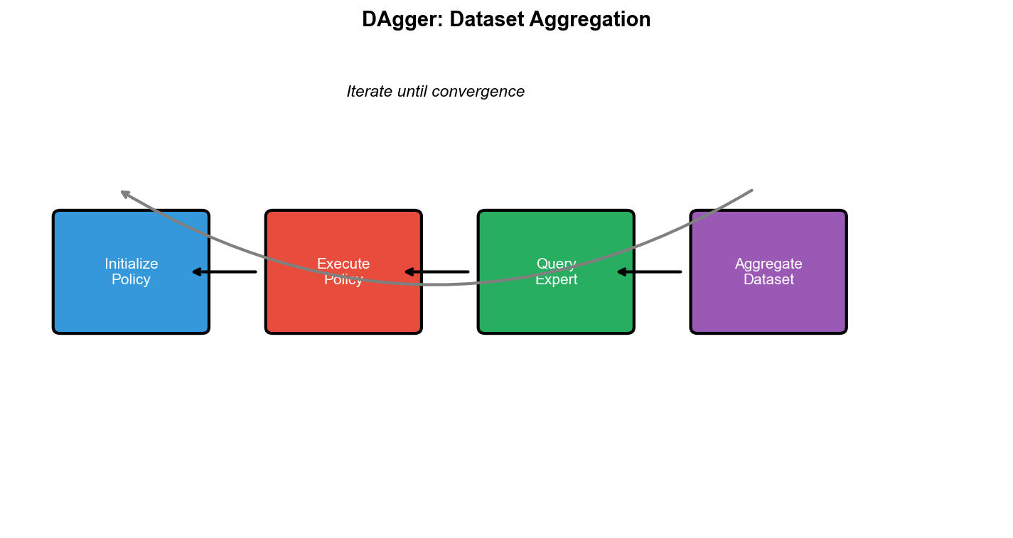
DAgger：数据集聚合

核心思想

DAgger（ Dataset Aggregation，数据集聚合）的核心思想很简单：

在学习过程中，用当前策略与环境交互，收集新的状态，然后查询专家在这些状态下会怎么做。

这样，即使策略犯了错误进入了新状态，我们也能获得专家在这些状态下的正确动作。

算法流程：

用专家策略收集初始数据集$_0 $训练初始策略$ _1 $对于$ i = 1, 2, ..., N $：用策略$ _i$ 与环境交互，收集状态序列 - 对每个状态，查询专家动作 - 将新数据加入数据集： - 在上重新训练策略 关键洞察：

DAgger 打破了分布漂移的恶性循环： - 策略犯错 → 进入新状态 → 获得专家标签 → 学会在新状态下正确行动

理论保证

DAgger 有严格的理论保证。设为训练误差（在训练集上的平均错误率），为轨迹长度。

定理（ Ross et al., 2011）：经过轮 DAgger 迭代后，策略满足：

J() - J(^*) (T)$$

与行为克隆的相比，这是线性而非二次的！

直觉理解： - 行为克隆的误差会累积和放大 - DAgger 通过覆盖所有可能访问的状态，将问题变成了"在每个状态上犯错的概率" - 每个时刻独立地有的错误概率，个时刻总共

详细实现

class DAgger:
    """
    DAgger (Dataset Aggregation) 算法
    
    通过迭代地收集数据来解决分布漂移问题：
    1. 用当前策略采集轨迹
    2. 查询专家获取这些状态的正确动作
    3. 将数据加入训练集
    4. 重新训练策略
    """
    
    def __init__(self, state_dim, action_dim, hidden_dims=[256, 256], 
                 lr=1e-3, continuous=False):
        """初始化 DAgger"""
        self.bc = BehavioralCloning(
            state_dim, action_dim, hidden_dims, lr, continuous
        )
        self.dataset = {'states': [], 'actions': []}
        self.continuous = continuous
        self.action_dim = action_dim
    
    def collect_data_with_expert(self, env, expert_policy, n_episodes,
                                  use_learner=True, beta=0.5):
        """
        收集数据：用学习者或混合策略采集轨迹，用专家标注动作
        
        Args:
            env: 环境
            expert_policy: 专家策略函数
            n_episodes: 收集的 episode 数
            use_learner: 是否使用学习者策略（ vs 纯专家）
            beta: 混合策略中专家的比例（安全学习时使用）
        
        Returns:
            new_states: 新收集的状态
            new_actions: 专家在这些状态下的动作
            episode_rewards: 每个 episode 的奖励（用真实执行动作）
        """
        new_states = []
        new_actions = []
        episode_rewards = []
        
        for ep in range(n_episodes):
            state = env.reset()
            done = False
            episode_reward = 0
            
            while not done:
                # 决定执行哪个动作
                if not use_learner:
                    # 纯专家数据收集
                    action = expert_policy(state)
                elif np.random.random() < beta:
                    # 混合策略：有 beta 概率用专家
                    action = expert_policy(state)
                else:
                    # 用学习者策略
                    action = self.bc.get_action(state)
                
                # 关键：无论执行什么动作，都记录专家的动作作为标签
                expert_action = expert_policy(state)
                
                new_states.append(state)
                new_actions.append(expert_action)
                
                # 环境交互
                next_state, reward, done, _ = env.step(action)
                state = next_state
                episode_reward += reward
            
            episode_rewards.append(episode_reward)
        
        return (np.array(new_states), np.array(new_actions), 
                episode_rewards)
    
    def train(self, env, expert_policy, n_iterations=10, 
              n_episodes_init=50, n_episodes_per_iter=20,
              epochs_per_iter=50, beta_schedule='linear'):
        """
        DAgger 训练主循环
        
        Args:
            env: 环境
            expert_policy: 专家策略
            n_iterations: 迭代轮数
            n_episodes_init: 初始数据收集的 episode 数
            n_episodes_per_iter: 每轮收集的 episode 数
            epochs_per_iter: 每轮训练的 epoch 数
            beta_schedule: 混合比例的调度策略
                - 'linear': 线性衰减
                - 'constant': 保持不变
                - 'exponential': 指数衰减
        """
        rewards_history = []
        
        # 第 0 轮：用专家收集初始数据
        print("Collecting initial expert data...")
        states, actions, _ = self.collect_data_with_expert(
            env, expert_policy, n_episodes_init, use_learner=False
        )
        self.dataset['states'].extend(states)
        self.dataset['actions'].extend(actions)
        
        # 训练初始策略
        all_states = np.array(self.dataset['states'])
        all_actions = np.array(self.dataset['actions'])
        self.bc.train(all_states, all_actions, epochs=epochs_per_iter)
        
        # DAgger 迭代
        for iteration in range(n_iterations):
            # 计算当前的 beta（混合比例）
            if beta_schedule == 'linear':
                beta = max(0.1, 1 - iteration / n_iterations)
            elif beta_schedule == 'exponential':
                beta = 0.5 ** (iteration + 1)
            else:  # constant
                beta = 0.5
            
            # 收集新数据
            states, actions, episode_rewards = self.collect_data_with_expert(
                env, expert_policy, n_episodes_per_iter,
                use_learner=True, beta=beta
            )
            
            # 聚合数据集
            self.dataset['states'].extend(states)
            self.dataset['actions'].extend(actions)
            
            # 在完整数据集上重新训练
            all_states = np.array(self.dataset['states'])
            all_actions = np.array(self.dataset['actions'])
            self.bc.train(all_states, all_actions, epochs=epochs_per_iter)
            
            # 评估当前策略
            eval_reward, _ = self.bc.evaluate(env, n_episodes=10)
            rewards_history.append(eval_reward)
            
            print(f"Iteration {iteration+1}: beta={beta:.2f}, "
                  f"dataset_size={len(self.dataset['states'])}, "
                  f"eval_reward={eval_reward:.2f}")
        
        return rewards_history
    
    def get_action(self, state):
        """获取动作"""
        return self.bc.get_action(state)

def create_expert_from_rl(env_name, expert_path=None):
    """
    创建专家策略（可以从预训练的 RL 模型加载）
    
    在实际应用中，专家可能是：
    - 人类操作员
    - 预训练的 RL 智能体
    - 基于规则的控制器
    """
    import gym
    env = gym.make(env_name)
    
    if expert_path:
        # 从文件加载
        expert = torch.load(expert_path)
    else:
        # 这里用一个简单的策略作为"专家"
        # 实际应用中应该用真正的专家
        class SimpleExpert:
            def __call__(self, state):
                # CartPole 的简单专家规则
                if state[2] > 0:  # 杆向右倾斜
                    return 1  # 向右推
                else:
                    return 0  # 向左推
        expert = SimpleExpert()
    
    return expert

DAgger 的变体

1. 安全 DAgger（ SafeDAgger）

在某些应用（如自动驾驶）中，让学习者完全控制可能很危险。 SafeDAgger 使用"护栏"机制：

def safe_dagger_step(state, learner, expert, safety_threshold):
    """安全的 DAgger 执行步骤"""
    learner_action = learner.get_action(state)
    expert_action = expert(state)
    
    # 计算学习者和专家动作的差异
    if continuous:
        diff = np.linalg.norm(learner_action - expert_action)
    else:
        diff = 0 if learner_action == expert_action else 1
    
    # 如果差异太大，使用专家动作（安全措施）
    if diff > safety_threshold:
        return expert_action, expert_action  # 执行专家，标注专家
    else:
        return learner_action, expert_action  # 执行学习者，标注专家

2. 样本高效 DAgger

不是每个状态都需要专家标注。可以选择性地查询： - 只在"不确定"的状态上查询（用 ensemble 模型衡量不确定性） - 只在"重要"的状态上查询（用优势函数或 TD 误差衡量）

3. HG-DAgger（ Human-Gated DAgger）

让人类专家决定何时介入：

def hgdagger_episode(env, learner, human_expert):
    """人类决定何时介入的 DAgger"""
    state = env.reset()
    done = False
    data = []
    
    while not done:
        learner_action = learner.get_action(state)
        
        # 显示给人类，询问是否需要修正
        human_action = human_expert.maybe_correct(state, learner_action)
        
        if human_action is not None:
            # 人类介入
            action = human_action
            data.append((state, human_action))
        else:
            # 人类认为学习者做得对
            action = learner_action
        
        state, _, done, _ = env.step(action)
    
    return data

DAgger 的局限性

需要交互式专家：在很多场景下，我们无法随时查询专家（专家可能是历史数据、已故的大师等）
专家负担重：专家需要对大量状态提供标签，这可能非常耗时
专家必须完美： DAgger 假设专家总是给出正确答案，但人类专家也会犯错或不一致
安全性：学习过程中可能访问危险状态

当我们无法使用交互式专家时，需要其他方法——逆强化学习和 GAIL 。

逆强化学习（ Inverse Reinforcement Learning）

问题设定与动机

前面的方法（ BC 和 DAgger）都是直接从状态到动作的映射。但有一个更深层的问题：专家为什么要这样做？

如果我们能理解专家的目标（奖励函数），我们就能： 1. 泛化到专家没有示范过的情况 2. 理解专家行为背后的"意图" 3. 在不同环境中应用相同的目标

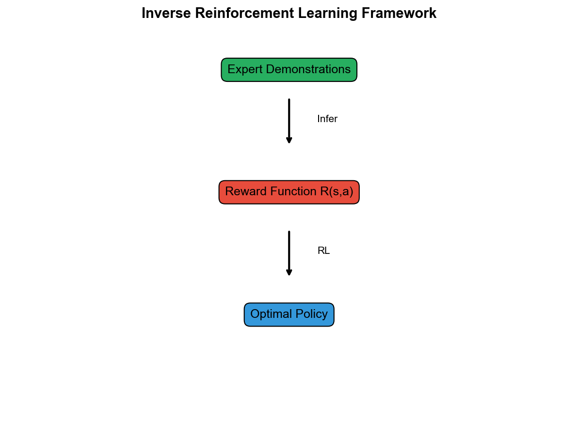
逆强化学习（ Inverse Reinforcement Learning, IRL）的思路是：

从专家示范中推断出奖励函数，然后用标准 RL 方法优化这个奖励。

形式化地，给定专家示范， IRL 寻找奖励函数使得： 1. 在下，专家策略是（接近）最优的 2. 专家策略比其他策略获得更高的累积奖励

奖励模糊性问题

IRL 的一个根本挑战是奖励模糊性：给定一组示范，可能有无穷多个一致的奖励函数！

例子：考虑最极端的情况——奖励函数恒为 0：。在这个奖励下，所有策略都是最优的（累积奖励都是 0），专家策略当然也是最优的。但这个奖励完全没有信息。

更一般地，任何能被专家策略最优化的奖励函数都是有效的。我们需要某种正则化或假设来选择"好"的奖励函数。

最大熵逆强化学习（ Maximum Entropy IRL）

最大熵 IRL（ Ziebart et al., 2008）通过一个优雅的假设解决了这个问题：

专家策略在所有"同样好"的选择中，偏好熵最大的那个。

换句话说，专家不会无缘无故地偏好某些动作——如果两个动作同样好，专家会随机选择。

这导致专家策略具有以下形式：

或者更一般地，对于整个轨迹：

P(| r) (_t r(s_t, a_t))$$

直觉：高奖励的轨迹被指数级地偏好，但不是确定性地选择最优轨迹。这是一种"软最优"。

目标函数

最大熵 IRL 的目标是最大化专家轨迹的似然：

展开概率：

P(| r_) = $$

其中是配分函数，对所有可能轨迹求积分。

因此目标变为：

梯度计算

对求梯度：

第二项可以写成：

其中是在当前奖励下的最优策略。

最终梯度：

$专家轨迹的特征当前策略轨迹的特征$

直觉解释： - 第一项：增加专家轨迹的奖励 - 第二项：减少当前策略轨迹的奖励 - 收敛时：两者相等，意味着当前策略与专家匹配

详细实现

import torch
import torch.nn as nn
import torch.optim as optim
import numpy as np

class MaxEntIRL:
    """
    最大熵逆强化学习
    
    从专家示范中学习奖励函数，然后用 RL 优化该奖励。
    
    核心思想：
    1. 假设专家策略是软最优的：π*(a|s) ∝ exp(Q*(s,a))
    2. 最大化专家轨迹的似然
    3. 梯度 = 专家特征期望 - 当前策略特征期望
    """
    
    def __init__(self, state_dim, action_dim, hidden_dim=128, 
                 reward_lr=1e-3, policy_lr=1e-3, continuous=False):
        """
        初始化 MaxEnt IRL
        
        Args:
            state_dim: 状态维度
            action_dim: 动作维度
            hidden_dim: 隐藏层维度
            reward_lr: 奖励网络学习率
            policy_lr: 策略网络学习率
            continuous: 是否是连续动作空间
        """
        self.state_dim = state_dim
        self.action_dim = action_dim
        self.continuous = continuous
        
        # 奖励网络： r(s, a) -> scalar
        self.reward_net = nn.Sequential(
            nn.Linear(state_dim + action_dim, hidden_dim),
            nn.ReLU(),
            nn.Linear(hidden_dim, hidden_dim),
            nn.ReLU(),
            nn.Linear(hidden_dim, 1)
        )
        self.reward_optimizer = optim.Adam(
            self.reward_net.parameters(), lr=reward_lr
        )
        
        # 策略网络
        if continuous:
            self.policy_mean = nn.Sequential(
                nn.Linear(state_dim, hidden_dim),
                nn.ReLU(),
                nn.Linear(hidden_dim, action_dim),
                nn.Tanh()
            )
            self.policy_log_std = nn.Parameter(torch.zeros(action_dim))
            policy_params = list(self.policy_mean.parameters()) + [self.policy_log_std]
        else:
            self.policy = nn.Sequential(
                nn.Linear(state_dim, hidden_dim),
                nn.ReLU(),
                nn.Linear(hidden_dim, action_dim),
                nn.Softmax(dim=-1)
            )
            policy_params = self.policy.parameters()
        
        self.policy_optimizer = optim.Adam(policy_params, lr=policy_lr)
        
        # 价值网络（用于 RL 内循环）
        self.value_net = nn.Sequential(
            nn.Linear(state_dim, hidden_dim),
            nn.ReLU(),
            nn.Linear(hidden_dim, 1)
        )
        self.value_optimizer = optim.Adam(self.value_net.parameters(), lr=1e-3)
    
    def compute_reward(self, states, actions):
        """计算奖励 r(s, a)"""
        if not isinstance(states, torch.Tensor):
            states = torch.FloatTensor(states)
        if not isinstance(actions, torch.Tensor):
            if self.continuous:
                actions = torch.FloatTensor(actions)
            else:
                # 将离散动作转换为 one-hot
                actions = torch.LongTensor(actions)
                actions = torch.nn.functional.one_hot(
                    actions, self.action_dim
                ).float()
        
        if len(states.shape) == 1:
            states = states.unsqueeze(0)
        if len(actions.shape) == 1:
            actions = actions.unsqueeze(0)
        
        inputs = torch.cat([states, actions], dim=-1)
        return self.reward_net(inputs).squeeze(-1)
    
    def get_action(self, state, deterministic=False):
        """从策略采样动作"""
        state = torch.FloatTensor(state).unsqueeze(0)
        
        if self.continuous:
            mean = self.policy_mean(state)
            if deterministic:
                return mean.squeeze().detach().numpy()
            std = torch.exp(self.policy_log_std)
            action = mean + std * torch.randn_like(mean)
            return action.squeeze().detach().numpy()
        else:
            probs = self.policy(state)
            if deterministic:
                return probs.argmax(dim=1).item()
            return torch.multinomial(probs, 1).item()
    
    def sample_trajectories(self, env, n_episodes=10, max_steps=200):
        """用当前策略采样轨迹"""
        trajectories = []
        
        for _ in range(n_episodes):
            states, actions, rewards = [], [], []
            state = env.reset()
            
            for _ in range(max_steps):
                action = self.get_action(state)
                next_state, _, done, _ = env.step(action)
                
                states.append(state)
                actions.append(action)
                
                # 用学习的奖励
                with torch.no_grad():
                    r = self.compute_reward(
                        np.array([state]), 
                        np.array([action])
                    ).item()
                rewards.append(r)
                
                state = next_state
                if done:
                    break
            
            trajectories.append({
                'states': np.array(states),
                'actions': np.array(actions),
                'rewards': np.array(rewards)
            })
        
        return trajectories
    
    def compute_feature_expectation(self, trajectories):
        """
        计算轨迹的特征期望（梯度）
        
        这是奖励函数的梯度，不是奖励值本身
        """
        total_grad = None
        n_samples = 0
        
        for traj in trajectories:
            states = torch.FloatTensor(traj['states'])
            if self.continuous:
                actions = torch.FloatTensor(traj['actions'])
            else:
                actions = torch.nn.functional.one_hot(
                    torch.LongTensor(traj['actions']), 
                    self.action_dim
                ).float()
            
            inputs = torch.cat([states, actions], dim=-1)
            rewards = self.reward_net(inputs).sum()
            
            self.reward_optimizer.zero_grad()
            rewards.backward()
            
            if total_grad is None:
                total_grad = [p.grad.clone() for p in self.reward_net.parameters()]
            else:
                for i, p in enumerate(self.reward_net.parameters()):
                    total_grad[i] += p.grad.clone()
            
            n_samples += len(traj['states'])
        
        # 平均
        for g in total_grad:
            g /= n_samples
        
        return total_grad
    
    def update_reward(self, expert_trajectories, policy_trajectories):
        """
        更新奖励函数
        
        梯度 = E_expert[∇ r] - E_policy[∇ r]
        """
        expert_grad = self.compute_feature_expectation(expert_trajectories)
        policy_grad = self.compute_feature_expectation(policy_trajectories)
        
        # 应用梯度
        self.reward_optimizer.zero_grad()
        for i, p in enumerate(self.reward_net.parameters()):
            # 注意：我们要最大化似然，所以是加不是减
            p.grad = policy_grad[i] - expert_grad[i]
        self.reward_optimizer.step()
    
    def update_policy_reinforce(self, env, n_episodes=10, 
                                 max_steps=200, gamma=0.99):
        """
        用 REINFORCE 更新策略
        
        在 IRL 中，这是内循环——对当前奖励函数优化策略
        """
        for _ in range(n_episodes):
            states, actions, rewards = [], [], []
            state = env.reset()
            
            for _ in range(max_steps):
                action = self.get_action(state)
                next_state, _, done, _ = env.step(action)
                
                states.append(state)
                actions.append(action)
                
                with torch.no_grad():
                    r = self.compute_reward(
                        np.array([state]), 
                        np.array([action])
                    ).item()
                rewards.append(r)
                
                state = next_state
                if done:
                    break
            
            # 计算回报
            returns = []
            G = 0
            for r in reversed(rewards):
                G = r + gamma * G
                returns.insert(0, G)
            returns = torch.FloatTensor(returns)
            returns = (returns - returns.mean()) / (returns.std() + 1e-8)
            
            # 策略梯度
            states = torch.FloatTensor(np.array(states))
            
            if self.continuous:
                actions = torch.FloatTensor(np.array(actions))
                mean = self.policy_mean(states)
                std = torch.exp(self.policy_log_std)
                dist = torch.distributions.Normal(mean, std)
                log_probs = dist.log_prob(actions).sum(dim=1)
            else:
                actions = torch.LongTensor(actions)
                probs = self.policy(states)
                log_probs = torch.log(probs.gather(1, actions.unsqueeze(1)).squeeze() + 1e-8)
            
            loss = -(log_probs * returns).mean()
            
            self.policy_optimizer.zero_grad()
            loss.backward()
            self.policy_optimizer.step()
    
    def train(self, env, expert_trajectories, n_iterations=100,
              n_policy_updates=10, n_sample_episodes=20):
        """
        MaxEnt IRL 训练主循环
        
        Args:
            env: 环境
            expert_trajectories: 专家轨迹列表
            n_iterations: 外循环迭代次数
            n_policy_updates: 每次外循环中策略更新的次数
            n_sample_episodes: 每次采样的轨迹数
        """
        for iteration in range(n_iterations):
            # 1. 用当前策略采样轨迹
            policy_trajectories = self.sample_trajectories(
                env, n_episodes=n_sample_episodes
            )
            
            # 2. 更新奖励函数
            self.update_reward(expert_trajectories, policy_trajectories)
            
            # 3. 对新奖励更新策略（内循环）
            for _ in range(n_policy_updates):
                self.update_policy_reinforce(env)
            
            # 评估
            if iteration % 10 == 0:
                # 计算专家和策略的平均奖励
                expert_reward = np.mean([
                    self.compute_reward(
                        traj['states'], traj['actions']
                    ).mean().item()
                    for traj in expert_trajectories
                ])
                policy_reward = np.mean([
                    self.compute_reward(
                        traj['states'], traj['actions']
                    ).mean().item()
                    for traj in policy_trajectories
                ])
                
                print(f"Iteration {iteration}: "
                      f"expert_reward={expert_reward:.4f}, "
                      f"policy_reward={policy_reward:.4f}")

IRL 的挑战与扩展

1. 计算复杂度

每次更新奖励后，需要重新训练策略（内循环）。这使得 IRL 比直接模仿学习慢很多。

2. 奖励塑形

学习到的奖励函数可能不是"真正"的奖励，只是能解释专家行为的一个函数。

3. 深度 IRL

现代方法用神经网络参数化奖励函数，可以处理高维状态。代表方法包括： - Deep MaxEnt IRL - Guided Cost Learning - AIRL (Adversarial IRL)

GAIL：生成对抗模仿学习

核心思想

GAIL（ Generative Adversarial Imitation Learning）将模仿学习与 GAN 结合，提供了一种端到端的解决方案。

核心思想是：

训练一个判别器来区分专家轨迹和策略生成的轨迹，同时训练策略来"欺骗"判别器。

这与 GAN 完全类似： - 生成器（ Generator）= 策略：生成轨迹 - 判别器（ Discriminator）= ：区分专家和生成轨迹

当策略成功欺骗判别器时，它的行为就与专家无法区分了——这正是模仿学习的目标！

数学形式化

GAIL 优化以下目标：

其中： - ：判别器，输出来自策略（而非专家）的概率 - ：策略的熵， - ：熵正则化系数

判别器的优化：

对于固定的，判别器想最大化区分能力。最优判别器为：

D^*(s, a) = $$

其中是策略的状态-动作占用度量。

策略的优化：

策略想最小化，即让判别器认为自己的轨迹是专家的。

关键洞察：判别器的输出可以作为奖励信号！

r(s, a) = -D(s, a)$$ - 如果（判别器认为是专家），则（正常） - 如果（判别器认为是策略），则（惩罚）

实际上，为了数值稳定，通常使用：

r(s, a) = -D(s, a) r(s, a) = (1 - D(s, a))$$

与 IRL 的关系

GAIL 可以被视为隐式的 IRL：

传统 IRL：显式学习奖励函数，然后求解 RL
GAIL：判别器隐式地定义了奖励函数，并与策略联合优化

Ho & Ermon (2016)证明， GAIL 与最大熵 IRL 在占用度量匹配的意义上是等价的。

详细实现

import torch
import torch.nn as nn
import torch.optim as optim
import numpy as np
from torch.distributions import Categorical, Normal

class GAIL:
    """
    生成对抗模仿学习 (Generative Adversarial Imitation Learning)
    
    核心思想：
    1. 判别器学习区分专家和策略生成的(s,a)对
    2. 策略学习欺骗判别器
    3. 判别器的输出作为策略的奖励信号
    4. 用 PPO 优化策略
    """
    
    def __init__(self, state_dim, action_dim, hidden_dim=256,
                 disc_lr=3e-4, policy_lr=3e-4, continuous=False):
        """
        初始化 GAIL
        
        Args:
            state_dim: 状态维度
            action_dim: 动作维度
            hidden_dim: 隐藏层维度
            disc_lr: 判别器学习率
            policy_lr: 策略学习率
            continuous: 是否是连续动作空间
        """
        self.state_dim = state_dim
        self.action_dim = action_dim
        self.continuous = continuous
        
        # 判别器： D(s, a) -> [0, 1]
        # 输出接近 1 表示来自策略，接近 0 表示来自专家
        disc_input_dim = state_dim + (action_dim if continuous else action_dim)
        self.discriminator = nn.Sequential(
            nn.Linear(disc_input_dim, hidden_dim),
            nn.Tanh(),
            nn.Linear(hidden_dim, hidden_dim),
            nn.Tanh(),
            nn.Linear(hidden_dim, 1),
            nn.Sigmoid()
        )
        self.disc_optimizer = optim.Adam(
            self.discriminator.parameters(), lr=disc_lr
        )
        
        # 策略网络
        if continuous:
            self.policy_mean = nn.Sequential(
                nn.Linear(state_dim, hidden_dim),
                nn.Tanh(),
                nn.Linear(hidden_dim, hidden_dim),
                nn.Tanh(),
                nn.Linear(hidden_dim, action_dim),
                nn.Tanh()
            )
            self.policy_log_std = nn.Parameter(torch.zeros(action_dim))
            policy_params = list(self.policy_mean.parameters()) + [self.policy_log_std]
        else:
            self.policy = nn.Sequential(
                nn.Linear(state_dim, hidden_dim),
                nn.Tanh(),
                nn.Linear(hidden_dim, hidden_dim),
                nn.Tanh(),
                nn.Linear(hidden_dim, action_dim),
                nn.Softmax(dim=-1)
            )
            policy_params = self.policy.parameters()
        
        self.policy_optimizer = optim.Adam(policy_params, lr=policy_lr)
        
        # 价值网络（用于 PPO）
        self.value = nn.Sequential(
            nn.Linear(state_dim, hidden_dim),
            nn.Tanh(),
            nn.Linear(hidden_dim, hidden_dim),
            nn.Tanh(),
            nn.Linear(hidden_dim, 1)
        )
        self.value_optimizer = optim.Adam(self.value.parameters(), lr=policy_lr)
    
    def get_action(self, state, deterministic=False):
        """采样动作"""
        state = torch.FloatTensor(state).unsqueeze(0)
        
        if self.continuous:
            mean = self.policy_mean(state)
            if deterministic:
                return mean.squeeze().detach().numpy()
            std = torch.exp(self.policy_log_std)
            dist = Normal(mean, std)
            action = dist.sample()
            log_prob = dist.log_prob(action).sum(dim=-1)
            return action.squeeze().detach().numpy(), log_prob.detach()
        else:
            probs = self.policy(state)
            if deterministic:
                return probs.argmax(dim=1).item()
            dist = Categorical(probs)
            action = dist.sample()
            return action.item(), dist.log_prob(action).detach()
    
    def get_disc_input(self, states, actions):
        """准备判别器的输入"""
        if not isinstance(states, torch.Tensor):
            states = torch.FloatTensor(states)
        
        if self.continuous:
            if not isinstance(actions, torch.Tensor):
                actions = torch.FloatTensor(actions)
        else:
            if not isinstance(actions, torch.Tensor):
                actions = torch.LongTensor(actions)
            actions = torch.nn.functional.one_hot(
                actions, self.action_dim
            ).float()
        
        return torch.cat([states, actions], dim=-1)
    
    def compute_gail_reward(self, states, actions):
        """
        计算 GAIL 奖励
        
        r(s, a) = -log(D(s, a))
        
        D 接近 0（像专家）-> 奖励低（好）
        D 接近 1（像策略）-> 奖励高（惩罚）
        
        实际使用 log(1-D)更稳定
        """
        disc_input = self.get_disc_input(states, actions)
        
        with torch.no_grad():
            d = self.discriminator(disc_input)
            # 使用 log(1-D+eps)作为奖励，避免 log(0)
            rewards = torch.log(1 - d + 1e-8).squeeze()
        
        return rewards.numpy()
    
    def update_discriminator(self, expert_states, expert_actions,
                              policy_states, policy_actions,
                              n_updates=1):
        """
        更新判别器
        
        目标：区分专家和策略生成的(s,a)对
        - 专家数据标签： 0（ D 输出应该低）
        - 策略数据标签： 1（ D 输出应该高）
        """
        expert_input = self.get_disc_input(expert_states, expert_actions)
        policy_input = self.get_disc_input(policy_states, policy_actions)
        
        # 创建数据加载器用于 mini-batch
        n_expert = len(expert_states)
        n_policy = len(policy_states)
        batch_size = min(64, n_expert, n_policy)
        
        total_loss = 0
        for _ in range(n_updates):
            # 随机采样
            expert_idx = np.random.choice(n_expert, batch_size, replace=False)
            policy_idx = np.random.choice(n_policy, batch_size, replace=False)
            
            expert_batch = expert_input[expert_idx]
            policy_batch = policy_input[policy_idx]
            
            # 判别器预测
            expert_pred = self.discriminator(expert_batch)
            policy_pred = self.discriminator(policy_batch)
            
            # 二元交叉熵损失
            # 专家标签是 0，策略标签是 1
            expert_loss = -torch.log(1 - expert_pred + 1e-8).mean()
            policy_loss = -torch.log(policy_pred + 1e-8).mean()
            
            disc_loss = expert_loss + policy_loss
            
            self.disc_optimizer.zero_grad()
            disc_loss.backward()
            self.disc_optimizer.step()
            
            total_loss += disc_loss.item()
        
        return total_loss / n_updates
    
    def compute_gae(self, rewards, values, dones, gamma=0.99, lam=0.95):
        """计算 GAE 优势估计"""
        advantages = []
        gae = 0
        
        for t in reversed(range(len(rewards))):
            if t == len(rewards) - 1:
                next_value = 0
            else:
                next_value = values[t + 1]
            
            delta = rewards[t] + gamma * next_value * (1 - dones[t]) - values[t]
            gae = delta + gamma * lam * (1 - dones[t]) * gae
            advantages.insert(0, gae)
        
        return torch.FloatTensor(advantages)
    
    def update_policy_ppo(self, states, actions, old_log_probs, rewards, dones,
                           gamma=0.99, lam=0.95, eps_clip=0.2, 
                           c1=0.5, c2=0.01, n_epochs=10):
        """
        用 PPO 更新策略
        
        Args:
            states: 状态
            actions: 动作
            old_log_probs: 旧策略的对数概率
            rewards: GAIL 奖励
            dones: 终止标志
            gamma: 折扣因子
            lam: GAE lambda
            eps_clip: PPO 裁剪参数
            c1: 价值损失系数
            c2: 熵系数
            n_epochs: 每批数据的更新轮数
        """
        states = torch.FloatTensor(np.array(states))
        if self.continuous:
            actions = torch.FloatTensor(np.array(actions))
        else:
            actions = torch.LongTensor(actions)
        old_log_probs = torch.stack(old_log_probs)
        rewards = torch.FloatTensor(rewards)
        
        # 计算优势
        with torch.no_grad():
            values = self.value(states).squeeze().numpy()
        advantages = self.compute_gae(rewards.numpy(), values, dones, gamma, lam)
        returns = advantages + torch.FloatTensor(values)
        advantages = (advantages - advantages.mean()) / (advantages.std() + 1e-8)
        
        # PPO 更新
        for _ in range(n_epochs):
            # 当前策略的 log 概率和熵
            if self.continuous:
                mean = self.policy_mean(states)
                std = torch.exp(self.policy_log_std)
                dist = Normal(mean, std)
                log_probs = dist.log_prob(actions).sum(dim=-1)
                entropy = dist.entropy().sum(dim=-1).mean()
            else:
                probs = self.policy(states)
                dist = Categorical(probs)
                log_probs = dist.log_prob(actions)
                entropy = dist.entropy().mean()
            
            # 概率比
            ratios = torch.exp(log_probs - old_log_probs)
            
            # PPO-Clip 目标
            surr1 = ratios * advantages
            surr2 = torch.clamp(ratios, 1 - eps_clip, 1 + eps_clip) * advantages
            policy_loss = -torch.min(surr1, surr2).mean()
            
            # 价值损失
            value_pred = self.value(states).squeeze()
            value_loss = ((value_pred - returns) ** 2).mean()
            
            # 总损失
            loss = policy_loss + c1 * value_loss - c2 * entropy
            
            # 更新策略
            self.policy_optimizer.zero_grad()
            loss.backward()
            if self.continuous:
                nn.utils.clip_grad_norm_(
                    list(self.policy_mean.parameters()) + [self.policy_log_std],
                    0.5
                )
            else:
                nn.utils.clip_grad_norm_(self.policy.parameters(), 0.5)
            self.policy_optimizer.step()
        
        # 更新价值函数
        for _ in range(n_epochs):
            value_pred = self.value(states).squeeze()
            value_loss = ((value_pred - returns) ** 2).mean()
            
            self.value_optimizer.zero_grad()
            value_loss.backward()
            self.value_optimizer.step()
        
        return policy_loss.item(), value_loss.item(), entropy.item()
    
    def train(self, env, expert_states, expert_actions, 
              n_iterations=500, n_episodes_per_iter=10,
              max_steps=200, disc_updates_per_iter=3):
        """
        GAIL 训练主循环
        
        Args:
            env: 环境
            expert_states: 专家状态数组
            expert_actions: 专家动作数组
            n_iterations: 总迭代次数
            n_episodes_per_iter: 每轮采集的 episode 数
            max_steps: 每个 episode 最大步数
            disc_updates_per_iter: 每轮判别器更新次数
        """
        rewards_history = []
        
        for iteration in range(n_iterations):
            # 1. 用当前策略收集轨迹
            policy_states, policy_actions = [], []
            all_log_probs, all_rewards, all_dones = [], [], []
            episode_true_rewards = []
            
            for _ in range(n_episodes_per_iter):
                ep_states, ep_actions, ep_log_probs, ep_dones = [], [], [], []
                state = env.reset()
                ep_true_reward = 0
                
                for _ in range(max_steps):
                    action, log_prob = self.get_action(state)
                    next_state, reward, done, _ = env.step(action)
                    
                    ep_states.append(state)
                    ep_actions.append(action)
                    ep_log_probs.append(log_prob)
                    ep_dones.append(done)
                    ep_true_reward += reward
                    
                    state = next_state
                    if done:
                        break
                
                policy_states.extend(ep_states)
                policy_actions.extend(ep_actions)
                all_log_probs.extend(ep_log_probs)
                all_dones.extend(ep_dones)
                episode_true_rewards.append(ep_true_reward)
            
            # 2. 计算 GAIL 奖励
            gail_rewards = self.compute_gail_reward(
                np.array(policy_states), 
                np.array(policy_actions)
            )
            all_rewards = list(gail_rewards)
            
            # 3. 更新判别器
            n_samples = min(len(policy_states), len(expert_states))
            expert_idx = np.random.choice(
                len(expert_states), n_samples, replace=False
            )
            
            disc_loss = self.update_discriminator(
                expert_states[expert_idx],
                expert_actions[expert_idx],
                np.array(policy_states[:n_samples]),
                np.array(policy_actions[:n_samples]),
                n_updates=disc_updates_per_iter
            )
            
            # 4. 用 PPO 更新策略
            policy_loss, value_loss, entropy = self.update_policy_ppo(
                policy_states, policy_actions, all_log_probs,
                all_rewards, all_dones
            )
            
            # 记录和打印
            avg_true_reward = np.mean(episode_true_rewards)
            rewards_history.append(avg_true_reward)
            
            if iteration % 10 == 0:
                print(f"Iter {iteration}: "
                      f"true_reward={avg_true_reward:.2f}, "
                      f"disc_loss={disc_loss:.4f}, "
                      f"policy_loss={policy_loss:.4f}, "
                      f"entropy={entropy:.4f}")
        
        return rewards_history
    
    def evaluate(self, env, n_episodes=10, render=False):
        """评估策略"""
        rewards = []
        for _ in range(n_episodes):
            state = env.reset()
            done = False
            episode_reward = 0
            while not done:
                if render:
                    env.render()
                action = self.get_action(state, deterministic=True)
                if isinstance(action, tuple):
                    action = action[0]
                state, reward, done, _ = env.step(action)
                episode_reward += reward
            rewards.append(episode_reward)
        return np.mean(rewards), np.std(rewards)

GAIL 的优势与局限

优势：

不需要显式奖励：判别器隐式学习奖励结构
端到端训练：策略和"奖励"联合优化，无需两阶段
样本高效：比 MaxEnt IRL 更高效
处理高维：可以处理高维状态和连续动作
理论保证：在占用度量匹配意义上有保证

局限：

需要环境交互：不能纯离线学习
训练不稳定： GAN 的训练本身就不稳定
模式崩溃：可能只学习专家行为的一部分
难以解释：没有显式的奖励函数

GAIL 的变体

1. AIRL（ Adversarial Inverse Reinforcement Learning）

AIRL 修改判别器结构，使其可以恢复出显式的奖励函数：

D(s, a, s') = $$

其中可以分解为奖励和 shaping 项： 2. VAIL（ Variational Adversarial Imitation Learning）

VAIL 使用变分信息瓶颈来改善训练稳定性。

3. SAM（ State-only Adversarial Mimicking）

当动作不可观测时（如从视频学习）， SAM 只使用状态匹配。

方法对比与选择指南

各方法全面对比

方法	交互式专家	环境交互	样本效率	实现复杂度	理论保证	可解释性
BC	不需要	不需要	高（但有漂移）	低	弱	中
DAgger	需要	需要	中高	低	强	中
MaxEnt IRL	不需要	需要	低	高	强	高
GAIL	不需要	需要	中	中	中	低

选择指南

选择行为克隆（ BC）当： - 有大量专家数据 - 任务相对简单（短时间范围） - 计算资源有限 - 不能与环境交互

选择 DAgger 当： - 可以随时查询专家 - 专家标注成本不高 - 需要处理长时间范围任务 - 需要理论保证

选择逆强化学习（ IRL）当： - 需要理解专家的目标 - 需要在不同环境中泛化 - 需要可解释的奖励函数 - 有充足的计算资源

选择 GAIL 当： - 无法查询专家 - 需要高质量模仿 - 有环境交互能力 - 状态/动作空间较大

高级话题

多模态专家行为

专家可能在同一状态下采取不同动作。例如，避开障碍物可以左转也可以右转。

标准 BC 会学习"平均"行为——可能直接撞向障碍物！

解决方案：

混合密度网络（ MDN）

class MDNPolicy(nn.Module):
    """混合密度网络：输出高斯混合分布"""
    def __init__(self, state_dim, action_dim, n_components=5, hidden_dim=128):
        super().__init__()
        self.n_components = n_components
        self.action_dim = action_dim
        
        self.shared = nn.Sequential(
            nn.Linear(state_dim, hidden_dim),
            nn.ReLU(),
            nn.Linear(hidden_dim, hidden_dim),
            nn.ReLU()
        )
        
        # 混合权重
        self.pi_layer = nn.Linear(hidden_dim, n_components)
        # 每个组件的均值和方差
        self.mu_layer = nn.Linear(hidden_dim, n_components * action_dim)
        self.sigma_layer = nn.Linear(hidden_dim, n_components * action_dim)
    
    def forward(self, state):
        h = self.shared(state)
        
        pi = torch.softmax(self.pi_layer(h), dim=-1)  # 混合权重
        mu = self.mu_layer(h).view(-1, self.n_components, self.action_dim)
        sigma = torch.exp(self.sigma_layer(h)).view(-1, self.n_components, self.action_dim)
        
        return pi, mu, sigma
    
    def sample(self, state):
        pi, mu, sigma = self(state)
        
        # 选择组件
        k = torch.multinomial(pi, 1).squeeze()
        
        # 从选中的组件采样
        action = mu[range(len(mu)), k] + sigma[range(len(sigma)), k] * torch.randn_like(mu[0, 0])
        return action

条件 VAE（ CVAE）

学习潜在的行为模式，然后条件生成：3. Info-GAIL

在 GAIL 中加入潜在变量，学习不同的行为模式。

从次优示范学习

现实中，专家示范往往不是最优的。如何处理？

1. 加权行为克隆

给高质量示范更高权重：

def weighted_bc_loss(predictions, expert_actions, quality_scores):
    """
    加权行为克隆损失
    
    quality_scores: 每个示范的质量分数（可以是回报、评分等）
    """
    weights = torch.softmax(quality_scores / temperature, dim=0)
    losses = criterion(predictions, expert_actions)
    return (weights * losses).sum()

2. 排序学习

不是学习绝对的好动作，而是学习哪个动作比哪个更好：

P(a_1 a_2 | s) = (f(s, a_1) - f(s, a_2))$$

3. 自我改进（ Self-Improvement）

先模仿，再用 RL 自我提升：

def iterative_improvement(bc_agent, env, n_rounds=5):
    """迭代自我改进"""
    for round in range(n_rounds):
        # 用当前策略收集数据
        trajectories = collect_trajectories(bc_agent, env)
        
        # 筛选好的轨迹
        good_trajectories = filter_by_return(trajectories, top_k=0.2)
        
        # 重新训练
        bc_agent.train(good_trajectories)

跨域模仿学习

当专家和学习者的状态/动作空间不同时：

1. 第三人称模仿学习

从视频（第三人称视角）学习，但执行时是第一人称视角。

2. 跨形态迁移

机器人 A 演示，机器人 B 模仿（不同的身体结构）。

3. 领域自适应

对齐不同域的状态表示。

实践建议

数据收集

数据质量比数量更重要
确保覆盖多样化的场景
记录专家的"恢复"行为（从错误中纠正）
避免示范中的明显错误

训练技巧

状态归一化：对输入状态进行标准化
数据增强：加噪声、裁剪、旋转等
正则化： Dropout 、 L2 正则化防止过拟合
早停：监控验证集性能

评估方法

轨迹相似度：与专家轨迹的距离
任务成功率：完成任务的比例
累积奖励：在环境中获得的总奖励
人类评估：让人类评判行为质量

总结

模仿学习提供了一种不依赖显式奖励函数的学习范式，通过观察专家示范来学习策略：

行为克隆简单直接，但受分布漂移困扰，适合短时间任务和有大量数据的场景
DAgger通过交互式学习缓解漂移，需要可查询的专家，有理论保证
逆强化学习恢复奖励函数，提供可解释性和泛化能力，但计算昂贵
GAIL用对抗训练实现端到端模仿，是当前最流行的方法，平衡了性能和实现复杂度

这些方法各有优劣，选择取决于具体应用场景：是否有交互式专家、是否需要环境交互、对可解释性的需求、计算资源等。

模仿学习在机器人、自动驾驶、游戏 AI 、对话系统等领域有广泛应用。它与强化学习互补——当奖励函数难以定义时，模仿学习提供了另一条路径；而当需要超越专家时，强化学习更为适合。两者的结合（如用模仿学习初始化、用 RL 微调）往往能取得最好的效果。

下一章，我们将学习AlphaGo 与蒙特卡洛树搜索——看看如何结合深度学习与传统规划方法，在围棋这样的复杂游戏中达到超人水平。

参考文献

Pomerleau, D. A. (1989). ALVINN: An Autonomous Land Vehicle in a Neural Network. NIPS.
Ross, S., Gordon, G., & Bagnell, D. (2011). A Reduction of Imitation Learning and Structured Prediction to No-Regret Online Learning. AISTATS.
Ziebart, B. D., et al. (2008). Maximum Entropy Inverse Reinforcement Learning. AAAI.
Ho, J., & Ermon, S. (2016). Generative Adversarial Imitation Learning. NIPS.
Fu, J., Luo, K., & Levine, S. (2018). Learning Robust Rewards with Adversarial Inverse Reinforcement Learning. ICLR.
Abbeel, P., & Ng, A. Y. (2004). Apprenticeship Learning via Inverse Reinforcement Learning. ICML.
Finn, C., Levine, S., & Abbeel, P. (2016). Guided Cost Learning: Deep Inverse Optimal Control via Policy Optimization. ICML.

Q&A：常见问题解答

Q1: 模仿学习和监督学习有什么区别？

A: 主要区别在于数据分布。监督学习假设训练和测试数据来自同一分布（ i.i.d.假设），但模仿学习中，测试时的状态分布取决于学习到的策略，与训练时的专家状态分布不同。这就是分布漂移问题的根源。

Q2: 如何判断专家数据量是否足够？

A: 可以通过以下方式判断： - 学习曲线：增加数据是否还能提升性能 - 验证集误差：是否接近训练集误差（过拟合检查） - 状态空间覆盖：是否覆盖了可能遇到的状态

Q3: GAIL 训练不稳定怎么办？

A: 尝试以下方法： - 调整判别器和策略的更新频率（通常判别器更新更频繁） - 使用梯度惩罚或谱归一化稳定判别器 - 降低学习率 - 增加熵正则化系数 - 使用 WGAN 变体

Q4: 什么时候用 BC，什么时候用 GAIL？

A: BC 适合：简单任务、大量数据、无法与环境交互。 GAIL 适合：复杂任务、有限数据、可以与环境交互。如果可以用 BC 解决，优先用 BC（更简单、更快）。

Q5: 如何处理专家示范中的噪声和错误？

A: - 数据清洗：过滤明显的错误示范 - 加权学习：给高质量示范更高权重 - 排序学习：学习相对偏好而非绝对动作 - 鲁棒损失函数：如 Huber 损失对异常值更鲁棒

Q6: 模仿学习能超越专家吗？

A: 纯模仿学习理论上不能超越专家（目标就是复制专家）。但可以： - 用模仿学习初始化，然后用 RL 微调 - 聚合多个专家的优点 - 在专家表现不佳的状态上自我改进

Q7: 多专家情况如何处理？

A: - 如果专家策略相似：直接混合数据 - 如果专家风格不同：学习多模态策略（ MDN 、 CVAE） - 如果专家水平不同：加权或只用最好的专家

Q8: 如何评估模仿学习的效果？

A: 多角度评估： - 累积奖励（如果有奖励函数） - 与专家轨迹的相似度 - 任务成功率 - 人类主观评价 - 在分布外状态的鲁棒性